Send your good work in the knowledge base is simple. Use the form below

Students, graduate students, young scientists using the knowledge base in their studies and work will be very grateful to you.

Posted on http:// www. allbest. ru/

MINISTRY OF EDUCATION AND SCIENCE OF THE RUSSIAN FEDERATION

FEDERAL STATE BUDGET EDUCATIONAL

INSTITUTION OF HIGHER EDUCATION

"SAMARA STATE TECHNICAL UNIVERSITY"

Faculty of correspondence

Department "Transport Processes and Technological Complexes"

COURSE PROJECT

by academic discipline

"Fundamentals of the performance of technical systems"

Completed:

N. D. Tsygankov

Checked:

O. M. Batishcheva

Samara 2017

ESSAY

The explanatory note contains: 26 printed pages, 3 figures, 5 tables, 1 annex and 7 sources used.

CAR, LADA GRANTA 2190, REAR SUSPENSION, ANALYSIS OF THE NODE DESIGN, STRUCTURING OF FACTORS AFFECTING THE DECREASE OF THE NODE OPERATING CAPACITY, DEFINITION OF INPUT TESTING, DETERMINATION OF PARAMETERS, DETERMINATION OF THE PARAMETER

The purpose of this work is to study the factors affecting the decrease in the performance of technical systems, as well as to gain knowledge about the quantitative assessment of marriage based on the results of incoming control.

Works on the study of theoretical material, as well as work with real details and samples of the systems under study were carried out. Based on the results of the incoming inspection, a number of tasks were performed: the distribution law, the scrap percentage and the volume of the sample set of products were determined to ensure the specified control accuracy.

INTRODUCTION

1. ANALYSIS OF THE FACTORS AFFECTING THE REDUCTION OF THE OPERATING CAPACITY OF TECHNICAL SYSTEMS

1.1 Rear suspension design

1.2 Structuring factors

1.3 Analysis of factors affecting the rear suspension of the Lada Granta 2190

1.4 Analysis of the influence of processes on changing the state of the rear suspension elements of the Lada Grants

ENTRANCE CONTROL RESULTS

2.1 The concept of incoming inspection, basic formulas

2.2 Checking for gross error

2.3 Determination of the number of intervals by subdividing the control setpoints

2.4 Building a histogram

2.5 Determination of the percentage of scrap in the party

CONCLUSION

LIST OF USED SOURCES

INTRODUCTION

In order to effectively manage the processes of changing the technical state of machines and justify measures aimed at reducing the intensity of wear of machine parts, it is necessary to determine the type of wear of surfaces in each specific case. For this, it is necessary to set the following characteristics: type of relative movement of surfaces (frictional contact scheme); the nature of the intermediate medium (type of lubricant or working fluid); main wear mechanism.

By the type of intermediate medium, wear is distinguished by friction without lubricant, by friction with lubricant, and by friction with abrasive material. Depending on the properties of the materials of the parts, lubricant or abrasive material, as well as on their quantitative ratio in the mates, in the process of work, there are surface destruction of various types.

In real operating conditions of machine interfaces, several types of wear are observed simultaneously. However, as a rule, it is possible to establish the leading type of wear, limiting the durability of parts, and to separate it from the rest, accompanying types of surface destruction, which insignificantly affect the performance of the interface. The mechanism of the main type of wear is determined by examining the worn surfaces. Observing the nature of the manifestation of wear of the friction surfaces (the presence of scratches, cracks, traces of chipping, destruction of the oxide film) and knowing the indicators of the properties of the materials of parts and lubricant, as well as data on the presence and nature of the abrasive, the intensity of wear and the mode of operation of the interface, it is possible to fully justify the conclusion about the type of wear of the interface and develop measures to increase the durability of the machine.

1. ANALYSIS OF FACTORS AFFECTING THE REDUCTION OF SLAVESABOUTCAPACITY OF TECHNICAL SYSTEMS

1.1 Rear suspension design

The suspension provides a resilient connection between the body and the wheels, softening shocks and impacts when the vehicle is driven over uneven roads. Thanks to its presence, the durability of the car increases, and the driver and passengers feel comfortable. The suspension has a positive effect on the stability and handling of the vehicle, its smoothness. On the Lada Granta car, the rear suspension repeats the design of the previous generations of LADA cars - the VAZ-2108 family, the VAZ-2110 family, Kalina and Priora. The rear suspension of the car is semi-independent, made on an elastic beam with trailing arms, coil springs and double-acting telescopic shock absorbers. The rear axle beam consists of two trailing arms connected by a U-cross member. This section provides the connector (cross member) with greater bending stiffness and less torsional stiffness. The connector allows the levers to move relative to each other within a small range. The levers are made of a tube of variable cross-section, this gives them the necessary rigidity. Brackets for mounting the shock absorber, the rear brake shield and the axle of the wheel hub are welded to the rear end of each lever. At the front, the beam levers are bolted into removable side member brackets. The mobility of the levers is provided by rubber-metal hinges (silent blocks) pressed into the front ends of the levers. The lower shock absorber eyelet attaches to the beam arm bracket. The shock absorber is attached to the body by a rod with a nut. The elasticity of the upper and lower joints of the shock absorber is provided by the rod cushions and a rubber-metal bushing pressed into the lug. The shock absorber rod is covered with a corrugated casing that protects it from dirt and moisture. In case of suspension breakdowns, the stroke of the shock absorber rod is delimited by a compression stroke buffer made of elastic plastic. The suspension spring with its lower coil rests on the support cup (a stamped steel plate welded to the shock absorber body), and the upper one rests against the body through a rubber gasket. The axle of the rear wheel hub is installed on the flange of the beam arm (it is fastened with four bolts). The hub with a double-row roller bearing pressed into it is held on the axle by a special nut. An annular collar is made on the nut, which reliably locks the nut by jamming it into the axle groove. The hub bearing is closed and does not require adjustment and lubrication during vehicle operation. Rear suspension springs are divided into two classes: A - more rigid, B - less rigid. Springs of class A are marked with brown paint, class B - blue. The springs of the same class must be installed on the right and left side of the vehicle. The springs of the same class are installed in the front and rear suspension. In exceptional cases, it is allowed to install class B springs in the rear suspension if the front has class A springs. Installation of class A springs on the rear suspension is not allowed if the front has class B springs.

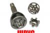
Fig. 1 Rear suspension Lada Granta 2190

1.2 Structuring factors

During the operation of the car, as a result of the impact on it of a number of factors (exposure to loads, vibrations, moisture, air flows, abrasive particles when dust and dirt hits the car, temperature effects, etc.), an irreversible deterioration of its technical condition occurs, associated with wear and tear of its parts, as well as a change in a number of their properties (elasticity, plasticity, etc.).

The change in the technical condition of the car is due to the operation of its components and mechanisms, the impact of external conditions and storage of the car, as well as random factors. Random factors include hidden defects in vehicle parts, structural overloads, etc.

The main permanent reasons for the change in the technical state of the car during its operation were wear, plastic deformation, fatigue, corrosion, as well as physicochemical changes in the material of parts (aging).

Wear is the process of destruction and separation of material from the surfaces of parts and (or) the accumulation of residual deformations during friction, which manifests itself in a gradual change in the size and (or) shape of interacting parts.

Wear is the result of the wear process of parts, expressed in changes in their size, shape, volume and weight.

Distinguish between dry and liquid friction. In dry friction, the friction surfaces of the parts interact directly with each other (for example, the friction of the brake pads on the brake drums or discs, or the friction of the clutch disc on the flywheel). This type of friction is accompanied by increased wear of the rubbing surfaces of the parts. With liquid (or hydrodynamic) friction between the rubbing surfaces of the parts, an oil layer is created that exceeds the microroughness of their surfaces and does not allow their direct contact (for example, the bearings of the crankshaft during steady-state operation), which dramatically reduces the wear of the parts. In practice, during the operation of most car mechanisms, the above main types of friction are constantly alternating and passing into each other, forming intermediate types.

The main types of wear are abrasive, oxidative, fatigue, erosion, as well as wear due to seizing, fretting and fretting corrosion.

Abrasive wear is a consequence of the cutting or scratching effect of solid abrasive particles (dust, sand) caught between the rubbing surfaces of the mating parts. Getting between the rubbing parts of open friction units (for example, between brake pads and discs or drums, between leaf springs, etc.), hard abrasive particles sharply increase their wear. In closed mechanisms (for example, in the crank mechanism of the engine), this type of friction is manifested to a much lesser extent and is a consequence of the ingress of abrasive particles into the lubricants and the accumulation of wear products in them (for example, when the oil filter and oil in the engine are not changed in time, when untimely replacement of damaged protective covers and grease in pivot joints, etc.).

Oxidative wear occurs as a result of the impact of an aggressive environment on the rubbing surfaces of mating parts, under the influence of which fragile oxide films are formed on them, which are removed by friction, and the exposed surfaces are again oxidized. This type of wear is observed on the parts of the cylinder-piston group of the engine, parts of the hydraulic brake and clutch cylinders.

Fatigue wear consists in the fact that the hard surface layer of the part material becomes brittle as a result of friction and cyclic loads and breaks down (crumbles), exposing the less hard and worn layer underneath. This type of wear occurs on the raceways of rolling bearing rings, gear teeth and gear wheels.

Erosive wear occurs as a result of the action on the surface of parts of high-speed fluid and (or) gas flows, with abrasive particles contained in them, as well as electrical discharges. Depending on the nature of the erosion process and the predominant effect on the details of certain particles (gas, liquid, abrasive), gas, cavitation, abrasive and electrical erosion are distinguished

Gas erosion consists in the destruction of the material of the part under the influence of mechanical and thermal effects of gas molecules. Gas erosion is observed on the valves, piston rings and the cylinder mirror of the engine, as well as on parts of the exhaust system.

Cavitation erosion of parts occurs when the continuity of the liquid flow is disrupted, when air bubbles are formed, which, bursting near the surface of the part, lead to numerous hydraulic shocks of the liquid against the metal surface and its destruction. Such damage affects engine parts that come into contact with the coolant: the inner cavities of the cooling jacket of the cylinder block, the outer surfaces of the cylinder liners, the cooling system pipes.

Electrical discharge wear is manifested in erosive wear of the surfaces of parts as a result of the effect of discharges when an electronic current passes, for example, between spark plug electrodes or breaker contacts.

Abrasive erosion occurs when the surface of parts is mechanically affected by abrasive particles contained in liquid flows (hydroabrasive erosion) and (or) gas (gaseous erosion), and is most typical for the outer parts of the car body (wheel arches, bottom, etc.). Wear when seizing occurs as a result of seizure, deep pulling out of the material of parts and its transfer from one surface to another, which leads to the appearance of scoring on the working surfaces of parts, to their jamming and destruction. Such wear occurs when local contacts occur between the rubbing surfaces, on which, due to excessive loads and speed, as well as a lack of lubrication, the oil film breaks, strong heating and "welding" of metal particles. A typical example is a crankshaft jam and liner rotation when the engine lubrication system malfunctions. Fretting wear is a mechanical wear of the contacting surfaces of parts with small oscillatory movements. If, in this case, under the influence of an aggressive environment, oxidative processes occur on the surfaces of the mating parts, then wear occurs during fretting corrosion. Such wear can occur, for example, at the points of contact between the liners of the crankshaft journals and their beds in the cylinder block and bearing caps.

Plastic deformation and destruction of car parts are associated with the achievement or exceeding of the yield or strength limits, respectively, for plastic (steel) or brittle (cast iron) materials of parts. These damages are usually the result of a violation of the rules for operating the vehicle (overloading, mismanagement, as well as a traffic accident). Sometimes plastic deformations of parts are preceded by their wear, leading to a change in the geometric dimensions and a decrease in the safety factor of the part.

Fatigue failure of parts occurs under cyclic loads that exceed the endurance limit of the part metal. In this case, there is a gradual formation and growth of fatigue cracks, leading, at a certain number of load cycles, to the destruction of the part. Such damage occurs, for example, on leaf springs and axle shafts during long-term operation of the vehicle under extreme conditions (prolonged overloads, low or high temperatures).

Corrosion occurs on the surfaces of parts as a result of chemical or electrochemical interaction of the material of the part with an aggressive environment, leading to oxidation (rusting) of the metal and, as a result, to a decrease in strength and deterioration of the appearance of parts. Salts used on the roads in winter and exhaust gases have the strongest corrosive effect on vehicle parts. Retention of moisture on metal surfaces strongly promotes corrosion, which is especially characteristic of hidden cavities and niches.

Aging is a change in the physical and chemical properties of materials of parts and operating materials during operation and during storage of a car or its parts under the influence of the external environment (heating or cooling, humidity, solar radiation). So, as a result of aging, industrial rubber goods lose their elasticity and crack, oxidative processes are observed in fuel, oils and operating fluids, which change their chemical composition and lead to a deterioration in their operational properties.

Changes in the technical condition of the vehicle are significantly influenced by the operating conditions: road conditions (technical category of the road, type and quality of the road surface, inclines, ups and downs, road curves), traffic conditions (heavy city traffic, traffic on country roads), climatic conditions ( ambient temperature, humidity, wind loads, solar radiation), seasonal conditions (dust in summer, dirt and moisture in autumn and spring), aggressive environment (sea air, salt on the road in winter, increasing corrosion), as well as transport conditions ( vehicle loading).

The main measures that reduce the rate of wear of parts during vehicle operation are: timely control and replacement of protective covers, as well as replacement or cleaning of filters (air, oil, fuel) that prevent abrasive particles from getting on the rubbing surfaces of parts; timely and high-quality performance of fastening, adjusting (adjusting valves and tension of the engine chain, wheel alignment angles, wheel bearings, etc.) and lubricants (replacing and adding oil in the engine, gearbox, rear axle, replacing and adding oil to the hubs wheels, etc.) works; timely restoration of the protective coating of the underbody, as well as the installation of wheel arches protecting the wheel arches.

To reduce corrosion of car parts and, first of all, the body, it is necessary to maintain their cleanliness, to carry out timely maintenance of the paintwork and its restoration, to carry out anti-corrosion treatment of the hidden cavities of the body and other parts subject to corrosion.

Serviceable is the condition of a car in which it meets all the requirements of regulatory and technical documentation. If the car does not meet at least one requirement of the regulatory and technical documentation, then it is considered faulty.

An operable state is a state of a car in which it meets only those requirements that characterize its ability to perform specified (transport) functions, i.e., a car is operable if it can transport passengers and goods without threatening traffic safety. A working car can be faulty, for example, it has a low oil pressure in the engine lubrication system, a deteriorated appearance, etc. If the car does not meet at least one of the requirements that characterize its ability to perform transport work, it is considered inoperative.

The transition of a car to a faulty, but operable state is called damage (violation of a good state), and into an inoperative state - a failure (violation of an operable state). performance wear deformation part

The limiting state of a car is a condition in which its further use for its intended purpose is unacceptable, economically impractical, or the restoration of its serviceability or operability is impossible or impractical. Thus, the vehicle enters the limit state when irreparable violations of safety requirements appear, the costs of its operation increase unacceptably, or there is an unrecoverable departure of technical characteristics beyond acceptable limits, as well as an unacceptable decrease in operating efficiency.

The vehicle's ability to resist the processes arising as a result of the aforementioned harmful environmental influences when the vehicle performs its functions, as well as its adaptability to restore its original properties, is determined and quantified using indicators of its reliability.

Reliability is a property of an object, including a car or its component part, to keep in time within the established limits the value of all parameters characterizing the ability to perform the required functions in specified modes and conditions of use, maintenance, repairs, storage and transportation. Reliability as a property characterizes and allows one to quantify, firstly, the current technical condition of the vehicle and its components, and secondly, how quickly their technical condition changes when operating under certain operating conditions.

Reliability is a complex property of a car and its component parts and includes the properties of reliability, durability, maintainability and storage.

1.3 Analysis of factors affecting the rear suspension of the Lada Granta 2190

Consider the factors affecting the decline in vehicle performance.

Any car can have faults and breakdowns, especially with regard to the suspension. This is because the suspension tolerates constant vibration when driving, softens shocks, and takes the entire weight of the car, including passengers and luggage, on itself. Based on this, Grant's liftback is more prone to breakage than the sedan, since the liftback body has a larger luggage compartment, designed for greater weight. The first problem encountered most often is the presence of knocking or extraneous noise. In this case, it is necessary to check the shock absorbers, as they need to be replaced in time, and can often fail. Also, the reason may be that the shock absorber mounting bolts are not fully tightened. Also, with a strong impact, not only the bushings, but also the racks themselves can be damaged. Then the repair will be more serious and expensive. The last reason for the suspension knocking may be a broken spring. (Fig. 2) In addition to knocking, it is necessary to check the suspension mechanism for leaks. If such traces are found, then this can indicate only one thing - a malfunction of the shock absorbers. If all the liquid flows out and the shock absorber dries up, then if it falls into the hole, the suspension will provide poor resistance, and the vibration from the impact will be very strong. The solution to this problem is quite simple - to replace the worn out element. The last malfunction that occurs on the Grant is when braking or accelerating, the car leads to the side. This indicates that on this side, one or two shock absorbers are worn out, and sag slightly more than the others. Because of this, the body is overweight.

1.4 Analysis of the influence of processes on changing the state of the rear suspension elements of the Lada Grants

To prevent accidents on the road, it is necessary to timely diagnose the vehicle as a whole and critical units in particular. The best and most qualified place to troubleshoot rear suspension problems is a car service center. You can also assess the technical condition of the suspension yourself while driving. When driving at low speed on uneven roads, the suspension should work without knocking, squeaking and other extraneous sounds. After driving over an obstacle, the vehicle must not sway.

Checking the suspension is best combined with checking the condition of tires and wheel bearings. One-sided tire tread wear indicates deformation of the rear suspension beam.

In this section, the factors influencing the decrease in vehicle performance were considered and analyzed. The influence of factors leads to a loss of performance of the unit and the vehicle as a whole, therefore it is necessary to carry out preventive measures to reduce the factors. After all, abrasive wear is a consequence of the cutting or scratching effect of solid abrasive particles (dust, sand) caught between the rubbing surfaces of the mating parts. Getting between the rubbing parts of the open friction units, hard abrasive particles sharply increase their wear.

Also, to prevent damage and increase the service life of the rear suspension, the rules for operating the car should be strictly observed, avoiding its operation at extreme modes and with overloads, this will extend the service life of critical parts.

2. QUANTITATIVE ASSESSMENT OF MARRIAGE IN A PARTY IN PESULTS OF INPUT CONTROL

2.1 The concept of incoming inspection, basic formulas

Quality control refers to checking the conformity of the quantitative or qualitative characteristics of a product or a process on which the quality of the product depends on the established technical requirements.

Product quality control is an integral part of the production process and is aimed at checking the reliability during its manufacture, consumption or operation.

The essence of product quality control at the enterprise is to obtain information about the state of the object and to compare the results obtained with the established requirements fixed in the drawings, standards, supply contracts, and technical specifications.

Control involves checking products at the very beginning of the production process and during the maintenance period, ensuring that in the event of deviations from the regulated quality requirements, corrective measures are taken to produce products of adequate quality, proper maintenance during operation and full satisfaction of customer requirements.

Input quality control of products should be understood as quality control of products intended for use in the manufacture, repair or operation of products.

The main tasks of incoming control can be:

Obtaining with high reliability an assessment of the quality of products submitted for control;

Ensuring unambiguity of mutual recognition of the results of product quality assessment carried out using the same methods and the same control plans;

Establishing the conformity of product quality to the established requirements in order to timely submit claims to suppliers, as well as to work promptly with suppliers to ensure the required level of product quality;

Preventing the launch into production or repair of products that do not meet the established requirements, as well as permission protocols according to GOST 2.124.

Quality control is one of the main functions in the quality management process. It is also the most voluminous function in terms of the methods used, to which a large number of works in various fields of knowledge are devoted. The importance of control lies in the fact that it allows you to identify errors in time, in order to quickly correct them with minimal losses.

Incoming control of product quality is understood as control of products received by the consumer and intended for use in the manufacture, repair or operation of products.

Its main purpose is to eliminate defects and conformity of products to the established values.

When conducting incoming control, plans and procedures for conducting statistical acceptance control of product quality on an alternative basis are used.

Methods and means used at the incoming inspection are selected taking into account the requirements for the accuracy of measuring the quality indicators of the controlled products. The departments of material and technical supply, external cooperation, together with the department of technical control, technical and legal services, form requirements for the quality and nomenclature of products supplied under contracts with supplier enterprises.

For any randomly selected product, it is impossible to determine in advance whether it will be reliable. Of two engines of the same brand, one may soon fail, and the second will be serviceable for a long time.

In this part of the course project, we will determine the quantitative assessment of the marriage in the batch based on the results of the incoming inspection using a Microsoft Excel spreadsheet. A table is given with the values \u200b\u200bof the operating time to the first failure due to the release of Lada Grant 2190 (table 1), this table will be the initial data for calculating the percentage of scrap and the volume of the sample number of products.

Table 2 Values \u200b\u200bof operating time to first failure

2.2 Checking for a gross error

Gross error (miss) is the error in the result of a single measurement included in a series of measurements, which for these conditions differs sharply from the rest of the results of this series. The source of gross errors can be abrupt changes in measurement conditions and errors made by the researcher. These include a breakdown of the device or a jolt, an incorrect reading on the scale of a measuring device, an incorrect recording of the observation result, chaotic changes in the parameters of the voltage supplying the measuring instrument, etc. Misses are immediately visible among the results obtained, because they are very different from the rest of the values. The presence of a miss can greatly distort the result of the experiment. But reckless discarding of sharply different measurements from other results can also lead to significant distortion of the measurement characteristics. Therefore, the initial processing of experimental data recommends checking any set of measurements for the presence of gross errors using the statistical three sigma test.

The three sigma criterion is applied to measurement results distributed according to the normal law. This criterion is reliable when the number of measurements n\u003e 20 ... 50. The arithmetic mean and standard deviation are calculated without taking into account the extreme (suspicious) values. In this case, the result is considered a gross error (miss) if the difference exceeds 3y.

The minimum and maximum sample values \u200b\u200bare checked for gross error.

In this case, all measurement results should be discarded whose deviations from the arithmetic mean exceed 3 , and the judgment on the variance of the general population is made on the basis of the remaining measurement results.

Method 3 showed that the minimum and maximum value of the initial data is not a gross error.

2.3 Determining the number of intervals by splitting the taskncontrol values

The choice of the optimal partitioning is essential for constructing a histogram, since with increasing intervals, the detail of the distribution density estimate decreases, and with decreasing, the accuracy of its value decreases. To select the optimal number of intervals n Sturges' rule is often applied.

Sturges' rule is an empirical rule for determining the optimal number of intervals into which the observed range of variation of a random variable is divided when constructing a histogram of its distribution density. Named for American statistician Herbert Sturges.

The resulting value is rounded to the nearest integer (Table 3).

Splitting into intervals is done in the following way:

The lower limit (n.a.) is defined as:

Table 3 Interval definition table



Average min
Average max
For MAX, for MIN
Dispersion

FOR For MIN
Dispersion

Gross error 3? (min)
Gross error 3? (max)
Number of intervals
Interval length

The upper limit (v.g.) Is defined as:

The subsequent lower bound will be equal to the upper of the previous interval.

The interval number, the values \u200b\u200bof the upper and lower boundaries are indicated in Table 4.

Table 4 Boundary definition table

Interval number

2.4 Plotting a histogram

To build a histogram, it is necessary to calculate the average value of the intervals and their average probability. The average value of the interval is calculated as:

The mean values \u200b\u200bof the interval and probability are presented in Table 5. The histogram is shown in Figure 3.

Table 5 Table of means and probabilities

Middle of interval	The number of incoming inspection results that fall within these boundaries	Probability

Fig. 3 Histogram

2.5 Determination of the percentage of scrap in the party

A defect is each individual non-conformity of a product with established requirements, and a product that has at least one defect is called defective ( marriage, defective products). Defect-free products are considered suitable.

The presence of a defect means that the actual value of the parameter (for example, Le) does not correspond to the specified normalized value of the parameter. Therefore, the condition for the absence of marriage is determined by the following inequality:

dmin? Ld? dmax,

where dmin, dmax - the smallest and largest maximum permissible values \u200b\u200bof the parameter that specify its tolerance.
The list, type and maximum permissible values \u200b\u200bof the parameters characterizing defects are determined by the quality indicators of the products and the data given in the regulatory and technical documentation of the enterprise for the manufactured products.

Distinguish correctable manufacturing defect and final manufacturing defect... Correctable includes products that are technically possible and economically feasible to correct in the conditions of the manufacturing enterprise; to the final - products with defects, the elimination of which is technically impossible or economically unprofitable. Such products must be disposed of as production waste, or sold by the manufacturer at a price significantly lower than the same product without defects ( discounted item).

By the time of detection, a manufacturing defect of products can be internal (identified at the production stage or in the factory warehouse) and external(found by the buyer or other person using this product, a defective product).

During operation, the parameters characterizing the performance of the system change from the initial (nominal) yn to the limit yp. If the parameter value is greater than or equal to ythe product is considered defective.

The limiting value of the parameter for nodes that ensure road safety is taken at a probability of b \u003d 15%, and for all other units and assemblies at b \u003d 5%.

The rear suspension is responsible for road safety, so the probability is b \u003d 15%.

When b \u003d 15%, the limit value is 16.5431, all products with a measured parameter equal to or higher than this value will be considered faulty

Thus, in the second section of the course project, the limit value of the controlled parameter was determined based on the error of the first kind.

CONCLUSION

In the first section of the course project, the influencing factors on the decrease in vehicle performance were considered and analyzed. The factors that directly affect the selected node - the ball joint were also considered. The influence of factors leads to a loss of performance of the unit and the vehicle as a whole, therefore it is necessary to carry out preventive measures to reduce the factors. After all, abrasive wear is a consequence of the cutting or scratching effect of solid abrasive particles (dust, sand) caught between the rubbing surfaces of the mating parts. Getting between the rubbing parts of open friction units, hard abrasive particles sharply increase their wear.

In the second section of the course project, the limit value of the controlled parameter was determined based on the error of the first kind.

LIST OF USED SOURCES

1. Collection of technological instructions for the maintenance and repair of the car Lada Granta JSC "Avtovaz", 2011, Togliatti

2. Avdeev M.V. and other Technology of repair of machines and equipment. - M .: Agropromizdat, 2007.

3. Borts A.D., Zakin J.Kh., Ivanov Yu.V. Diagnostics of the technical condition of the car. Moscow: Transport, 2008.159 p.

4. Gribkov V.M., Karpekin P.A. Reference book on equipment for maintenance and repair of cars. Moscow: Rosselkhozizdat, 2008.223 p.

Posted on Allbest.ru

...

"COURSE OF LECTURES ON THE DISCIPLINE" BASICS OF OPERATION OF TECHNICAL SYSTEMS "1. Basic provisions and dependences of reliability General dependencies ..."

COURSE OF LECTURES ON THE DISCIPLINE

"BASICS OF PERFORMANCE OF TECHNICAL

1. Basic provisions and dependences of reliability

Common dependencies

Significant dispersion of the main parameters of reliability predetermines

the need to consider it in a probabilistic aspect.

As shown above using the example of distribution characteristics,

reliability parameters are used in a statistical treatment for state assessment and in a probabilistic treatment for forecasting. The former are expressed in discrete numbers; in probability theory and the mathematical theory of reliability they are called valuations. With a sufficiently large number of tests, they are taken as true reliability characteristics.

Consider the tests carried out to assess the reliability or the operation of a significant number of N elements during time t (or operating time in other units). Let by the end of the test or service life there remain Np operable (non-failed) elements and n failed ones.

Then the relative number of failures is Q (t) \u003d n / N.

If the test is performed as a sample, then Q (t) can be considered as a statistical estimate of the probability of failure or, if N is large enough, as the probability of failure.

In the future, in cases where it is necessary to emphasize the difference between the probability estimate and the true probability value, the estimate will be additionally supplied with an asterisk, in particular Q * (t) n / N) Since uptime and failure are mutually opposite events, the sum of their probabilities is 1:

P (t)) + Q (t) \u003d 1.

The same follows from the above dependencies.

At t \u003d 0 n \u003d 0, Q (t) \u003d 0 and Р (t) \u003d 1.

For t \u003d n \u003d N, Q (t) \u003d 1 and P (t) \u003d 0.

The distribution of failures over time is characterized by the function of the density distribution f (t) of the time to failure. In () () the statistical interpretation f (t), in the probabilistic interpretation. Here \u003d n and Q are the increment in the number of failed objects and, accordingly, the probability of failures over time t.

The probabilities of failures and uptime in the density function f (t) are expressed by the dependencies Q (t) \u003d (); at t \u003d Q (t) \u003d () \u003d 1 P (t) \u003d 1 - Q (t) \u003d 1 - () \u003d 0 () o in (t), in contrast to the distribution density relative

- & nbsp– & nbsp–

Let us consider the reliability of the simplest design model of a system of series-connected elements, most typical for mechanical engineering (Fig. 1.2), in which the failure of each element causes a system failure, and the failures of the elements are assumed to be independent.

P1 (t) P2 (t) P3 (t)

- & nbsp– & nbsp–

Р (t) \u003d e (1 t1 + 2 t2) This dependence follows from the probability multiplication theorem.

To determine the failure rate on the basis of experiments, the mean time to failure is estimated mt \u003d where N is the total number of observations. Then \u003d 1 /.

Then, taking the logarithm of the expression for the probability of no-failure operation: lgР (t) \u003d

T lg e \u003d - 0.343 t, we conclude that the tangent of the angle of the straight line drawn through the experimental points is tg \u003d 0.343, whence \u003d 2.3tg With this method, there is no need to complete the test of all samples.

For the system Pst (t) \u003d e it. If 1 \u003d 2 \u003d… \u003d n, then Pst (t) \u003d enit. Thus, the probability of failure-free operation of a system consisting of elements with a probability of failure-free operation according to an exponential law also obeys an exponential law, and the failure rates of individual elements add up. Using the exponential distribution law, it is easy to determine the average number of products I that will fail at a given point in time, and the average number of products Np that will remain operational. At t0,1 n Nt; Np N (1 - t).

- & nbsp– & nbsp–

The distribution density curve is sharper and higher, the smaller S. It starts from t \u003d - and extends to t \u003d +;

- & nbsp– & nbsp–

Operations with a normal distribution are simpler than with others, so they are often replaced with other distributions. For small coefficients of variation S / m t, the normal distribution is a good substitute for binomial, Poisson and logarithmically normal.

The mathematical expectation and variance of the composition are respectively equal to m u \u003d m x + m y + m z; S2u \u003d S2x + S2y + S2z where mx, m y, m z - mathematical expectations of random variables;

1.5104 4104 Solution. Find the quantile up \u003d \u003d - 2.5; according to the table, we determine that P (t) \u003d 0.9938.

The distribution is characterized by the following function of the probability of failure-free operation (Fig.1.8) P (t) \u003d 0

- & nbsp– & nbsp–

Combined action of sudden and gradual failures The probability of failure-free operation of a product for a period t, if before that it has worked time T, according to the probability multiplication theorem is equal to P (t) \u003d Pv (t) Pn (t), where Pv (t) \u003d et and Pn (t) \u003d Pn (T + t) / Pn (T) - the probability of the absence of sudden and, accordingly, gradual failures.

- & nbsp– & nbsp–

2. Reliability of systems General information The reliability of most products in technology has to be determined when considering them as a system. Complex systems are divided into subsystems.

In terms of reliability, systems can be sequential, parallel and combined.

The most obvious example of sequential systems are automatic machine lines without redundant circuits and storage. In them, the name is realized literally. However, the concept of "sequential system" in reliability problems is broader than usual. These systems include all systems in which the failure of an element leads to a failure of the system. For example, the bearing system of mechanical transmissions is considered to be in series, although the bearings of each shaft run in parallel.

Examples of parallel systems are power systems of electrical machines running on a common grid, multi-engine aircraft, ships with two machines, and redundant systems.

Examples of combined systems are partially redundant systems.

Many systems consist of elements, the failures of each of which can be considered as independent. This consideration is widely used for operating failures and sometimes as a first approximation for parametric failures.

Systems can include elements, changing the parameters of which determines the failure of the system as a whole or even affects the performance of other elements. This group includes most of the systems when they are accurately considered for parametric failures. For example, the failure of precision metal-cutting machines according to the parametric criterion - loss of accuracy - is determined by the cumulative change in the accuracy of individual elements: the spindle assembly, guides, etc.

In a system with a parallel connection of elements, it is of interest to know the probability of failure-free operation of the entire system, i.e. of all its elements (or subsystems), a system without one, without two, etc. elements within the limits of the system's preservation of operability at least with strongly reduced indicators.

For example, a four-engine aircraft can continue flying after two engines fail.

The preservation of the performance of a system of identical elements is determined using the binomial distribution.

Consider a binomial m, where the exponent m is equal to the total number of parallel working elements; Р (t) and Q (t) are the probabilities of failure-free operation and, accordingly, failure of each of the elements.

We write down the results of the decomposition of binomials with exponents 2, 3, and 4, respectively, for systems with two, three and four parallel elements:

(P + Q) 2 \u003d P2 - \\ - 2PQ + Q2 \u003d 1;

(P + Q) 2 \u003d P3 + 3P2Q + 3PQ2 + Q3 \u003d 1;

(P + Q) 4 \u003d P4 + 4P3Q + 6P2Q2 + 4PQ3 + Q4 \u003d 1.

In them, the first terms express the probability of failure-free operation of all elements, the second - the probability of failure of one element and the failure-free operation of the rest, the first two terms - the probability of failure of no more than one element (no failure or failure of one element), etc. The last term expresses the probability of failure of all elements.

Convenient formulas for technical calculations of parallel redundant systems are given below.

The reliability of a system of series-connected elements obeying the Weibull distribution P1 (t) \u003d and P2 (t) \u003d also obeys the Weibull distribution P (t) \u003d 0, where the parameters m and t are rather complex functions of the arguments m1, m2, t01 and t02 ...

Using the method of statistical modeling (Monte Carlo) on a computer, graphs for practical calculations are constructed. The graphs allow you to determine the average resource (before the first failure) of a system of two elements in fractions of the average resource of an element with greater durability and the coefficient of variation for the system depending on the ratio of average resources and the coefficients of variation of elements.

For a system of three or more elements, you can use the graphs sequentially, and it is convenient to use them for elements in ascending order of their average resource.

It turned out that with the usual values \u200b\u200bof the coefficients of variation of the resources of the elements \u003d 0.2 ... 0.8, there is no need to take into account those elements whose average resource is five times or more greater than the average resource of the least durable element. It also turned out that in multi-element systems, even if average element resources are close to each other, there is no need to consider all elements. In particular, with the coefficient of variation of the resource of elements of 0.4, no more than five elements can be taken into account.

These provisions are largely applicable to systems subject to other closely related distributions.

Reliability of a sequential system under normal load distribution across systems If the load dissipation across the systems is negligible, and the load-bearing capacities of the elements are independent of each other, then the failures of the elements are statistically independent and therefore the probability P (RF0) of failure-free operation of the sequential system with the load-carrying capacity R under load F0 is the product of the probabilities of no-failure operation of the elements:

P (RF0) \u003d (Rj F0) \u003d, (2.1) where Р (Rj F0) is the probability of failure-free operation of the j-th element under load F0; n the number of elements in the system; FRj (F0) - the distribution function of the bearing capacity of the j-th element with the value of the random variable Rj equal to F0.

In most cases, the load has a significant dissipation across the systems, for example, universal machines (machine tools, cars, etc.) can be operated in different conditions. When the load is scattered across the systems, the estimate of the probability of system uptime P (RF) in the general case should be found by the formula of total probability, dividing the load distribution range into intervals F, finding for each load interval the product of the probability of uptime P (Rj Fi) for element at a fixed load on the probability of this load f (Fi) F, and then, summing these products over all intervals, P (RF) \u003d f (Fi) Fn P (Rj Fi) or, passing to integration, P (RF) \u003d (), (2.2) where f (F) - load distribution density; FRj (F) is the distribution function of the bearing capacity of the j-th element at the value of the bearing capacity Rj \u003d F.

Calculations according to formula (2.2) are generally laborious, since they involve numerical integration, and therefore, for large n, they are possible only on a computer.

In order not to calculate Р (R F) by formula (2.2), in practice, the probability of failure-free operation of systems Р (R Fmах) is often estimated at the maximum load Fmax possible. Take, in particular, Fmax \u003d mF (l + 3F), where mF is the mathematical expectation of the load and F is its coefficient of variation. This value Fmax corresponds to the largest value of the normally distributed random variable F over an interval equal to six standard deviations of the load. This method of assessing the reliability significantly underestimates the calculated indicator of the reliability of the system.

Below, a fairly accurate method is proposed for a simplified assessment of the reliability of a sequential system for the case of normal load distribution across systems. The idea of \u200b\u200bthe method is to approximate the distribution law of the bearing capacity of the system with a normal distribution so that the normal law is close to the true one in the range of reduced values \u200b\u200bof the bearing capacity of the system, since it is these values \u200b\u200bthat determine the value of the system reliability indicator.

Comparative calculations on a computer according to formula (2.2) (exact solution) and the proposed simplified method, given below, showed that its accuracy is sufficient for engineering calculations of the reliability of systems in which the coefficient of variation of the bearing capacity does not exceed 0.1 ... 0.15 , and the number of system elements does not exceed 10 ... 15.

The method itself is as follows:

1. Set by two values \u200b\u200bFA and FB of fixed loads. The formula (3.1) is used to calculate the probabilities of failure-free operation of the system at these loads. The loads are selected so that, when assessing the reliability of the system, the probability of failure-free operation of the system turns out to be within P (RFA) \u003d 0.45 ... 0.60 and P (R FA) \u003d 0.95 ... 0.99, i.e. ... would cover the interval of interest.

The approximate values \u200b\u200bof the loads can be taken close to the values \u200b\u200bFA (1 + F) mF, FB (1+ F) mF,

2. According to the table. 1.1 find the quantiles of the normal distribution upA and upB corresponding to the found probabilities.

3. The law of distribution of the bearing capacity of the system is approximated by a normal distribution with the parameters of the mathematical expectation mR and the coefficient of variation R. Let SR be the standard deviation of the approximating distribution. Then mR - FA + upASR \u003d 0 and mR - FB + upBSR \u003d 0.

From the above expressions, we obtain expressions for mR and R \u003d SR / mR:

R \u003d; (2.4)

4. The probability of failure-free operation of the system P (R F) for the case of normal distribution of the load F over systems with the parameters of the mathematical expectation m F and the coefficient of variation R is found in the usual way from the quantile of the normal distribution uр. The quantile uр is calculated by a formula reflecting the fact that the difference of two normally distributed random variables (the carrying capacity of the system and the load) is distributed normally with a mathematical expectation equal to the difference in their mathematical expectations and a root mean square equal to the root of the sum of the squares of their standard deviations:

up \u003d () 2 + where n \u003d m R / m F is the conditional safety factor based on the average values \u200b\u200bof the bearing capacity and load.

Let us consider the use of the described method by examples.

Example 1. It is required to estimate the probability of failure-free operation of a single-stage gearbox if the following is known.

Conditional safety margins for average values \u200b\u200bof bearing capacity and load are: gear 1 \u003d 1.5; input shaft bearings 2 \u003d 3 \u003d 1.4; bearings of the output shaft 4 \u003d 5 \u003d 1.6, the output and input shafts 6 \u003d 7 \u003d 2.0. This corresponds to the mathematical expectations of the bearing capacity of the elements 1 \u003d 1.5; 2 3 \u003d 1.4; 4 \u003d 5 \u003d 1.6;

6 \u003d 7 \u003d 2. Often in gearboxes n 6 and n7 and, accordingly, mR6 and mR7 are significantly larger. It is specified that the bearing capacities of the transmission, bearings and shafts are normally distributed with the same coefficients of variation 1 \u003d 2 \u003d… \u003d 7 \u003d 0.1, and the load on the gearboxes is also normally distributed with the coefficient of variation \u003d 0.1.

Decision. We set the loads FA and FB. We take FA \u003d 1.3, FB \u003d 1.1mF, assuming that these values \u200b\u200bwill give close to the required values \u200b\u200bof the probabilities of failure-free operation of systems at fixed loads P (R FA) and P (R FB).

We calculate the quantiles of the normal distribution of all elements corresponding to their probabilities of no-failure operation under loads FA and FB:

1 1,3 1,5 1 = = = - 1,34;

- & nbsp– & nbsp–

Using the table, we find the desired probability corresponding to the obtained quantile: (F) \u003d 0.965.

Example 2. For the conditions of the example considered above, we will find the probability of failure-free operation of the gearbox at maximum load in accordance with the methodology used earlier for practical calculations.

We take the maximum load Fmax \u003d TP (1 + 3F) \u003d mF (1 + 3 * 0.1) \u003d 1.3mF.

Decision. We calculate at this load the quantiles of the normal distribution of the probabilities of failure-free operation of the elements 1 \u003d - 1.333; 2 \u003d 3 \u003d -0.714;

4 = 5 = - 1,875; 8 = 7 = - 3,5.

According to the table, we find the probabilities P1 (R Fmax) \u003d 0.9087 corresponding to the quantiles;

P2 (R Fmax) \u003d P3 (R Fmax) \u003d 0.7624; P4 (R Fmax) \u003d P5 (R Fmax) \u003d 0.9695;

P6 (RFmax) \u003d P7 (R Fmax) \u003d 0.9998.

The probability of failure-free operation of the gearbox under load Pmax is calculated by formula (2.1). We get P (P ^ Pmax) \u003d 0.496.

Comparing the results of solving the two examples, we see that the first solution gives a reliability estimate that is much closer to the real one and higher than in the second example. The actual value of the probability, calculated on a computer according to formula (2.2), is 0.9774.

Assessment of the reliability of the system of the chain type Often, sequential systems are made up of the same elements (load or drive chain, gear with links, teeth, etc.). If the load is dissipated across the systems, then an approximate estimate of the system reliability can be obtained by the general method described in the previous paragraphs. Below we propose a more accurate and simple method for assessing reliability for a particular case of sequential systems - systems of the chain type with a normal distribution of the bearing capacity of the elements and the load over the systems.

The distribution law of the bearing capacity of a chain consisting of identical elements corresponds to the distribution of the minimum member of the sample, that is, a series of n numbers taken at random from the normal distribution of the bearing capacity of the elements.

This law differs from the normal one (Fig. 2.1) and is the more significant, the larger n. The mathematical expectation and standard deviation decrease with increasing n. In the theory of extreme distributions (the section of probability theory dealing with distributions of extreme members of samples), it is proved that the considered distribution with growth of n tends to double exponential. This limiting distribution law of the bearing capacity R of the chain P (R F 0), where F0 is the current value of the load, has the form P (R F0) R / \u003d eе. Here and (0) are distribution parameters. With real (small and medium) values \u200b\u200bof n, the double exponential distribution is unsuitable for use in engineering practice due to significant calculation errors.

The idea of \u200b\u200bthe proposed method is to approximate the distribution law of the bearing capacity of the system by a normal law.

The approximating and real distributions should be close both in the middle part and in the region of low probabilities (the left "tail" of the distribution density of the bearing capacity of the system), since it is this distribution region that determines the probability of the system's no-failure operation. Therefore, when determining the parameters of the approximating distribution, the equalities of the functions of the approximating and real distribution are put forward at the median value of the carrying capacity of the system corresponding to the probability of failure-free operation of the system.

After approximation, the probability of failure-free operation of the system, as usual, is found by the quantile of the normal distribution, which is the difference between two normally distributed random variables - the carrying capacity of the system and the load on it.

Let the laws of distribution of the bearing capacity of the elements Rk and the load on the system F be described by normal distributions with mathematical expectations, respectively, m Rk and m p and standard deviations S Rk and S F.

- & nbsp– & nbsp–

Taking into account that and depend on up, calculations by formulas (2.8) and (2.11) are performed by the method of successive approximations. As the first approximation to determine and take up \u003d - 1.281 (corresponding to P \u003d 0.900).

Reliability of systems with redundancy To achieve high reliability in mechanical engineering, structural, technological and operational measures may turn out to be insufficient, and then redundancy has to be used. This is especially true for complex systems for which the required high reliability of the system cannot be achieved by increasing the reliability of the elements.

Here, structural redundancy is considered, carried out by the introduction of redundant components into the system, which are redundant in relation to the minimum required structure of the object and perform the same functions as the main ones.

Redundancy reduces the probability of failures by several orders of magnitude.

Apply: 1) constant redundancy with loaded or hot standby; 2) redundancy by replacement with an unloaded or cold reserve; 3) redundancy with a reserve operating in lightweight mode.

Redundancy is most widely used in electronic equipment, in which the backup elements are small and easily switched.

Features of redundancy in mechanical engineering: in a number of systems, backup units are used as workers during peak hours; in a number of systems, redundancy ensures the preservation of operability, but with a decrease in performance.

Redundancy in its pure form in mechanical engineering is mainly used when there is a danger of accidents.

In transport vehicles, in particular in automobiles, a double or triple braking system is used; in trucks, double tires on the rear wheels.

Passenger airplanes use 3 ... 4 engines and several electric machines. The failure of one or even several machines, except for the last, does not lead to an aircraft accident. There are two cars in seagoing vessels.

The number of escalators and steam boilers is selected taking into account the possibility of failure and the need for repair. At the same time, all escalators can operate during peak hours. In general mechanical engineering, in critical units, a double lubrication system, double and triple seals are used. In the machines, spare sets of special tools are used. In factories, unique machines of the main production are trying to have two or more copies. In automatic production, storage devices, backup machines and even duplicate sections of automatic lines are used.

The use of spare parts in warehouses, spare wheels on cars can also be considered as a type of redundancy. Redundancy (general) should also include the design of a fleet of machines (for example, cars, tractors, machine tools), taking into account the time of their downtime for repair.

With a constant cut-out, the reserve elements or circuits are connected in parallel with the main ones (Fig. 2.3). The probability of failure of all elements (main and backup) according to the probability multiplication theorem Qst (t) \u003d Q1 (t) * Q2 (t) *… Qn (t) \u003d (), where Qi (t) is the probability of failure of element i.

Probability of no-failure operation Pst (t) \u003d 1 - Qst (t) If the elements are the same, then Qst (t) \u003d 1 (t) and Pst (t) \u003d 1 (t).

For example, if Q1 \u003d 0.01 and n \u003d 3 (double redundancy), then Pst \u003d 0.999999.

Thus, in systems with series-connected elements, the probability of failure-free operation is determined by multiplying the probabilities of failure-free operation of the elements, and in a system with parallel connection, the probability of failure is determined by multiplying the probabilities of failure of the elements.

If in the system (Fig. 2.5, a, b) a elements are not duplicated, and b elements are duplicated, then the reliability of the system Pst (t) \u003d Pa (t) Pb (t); Pa (t) \u003d (); Pb (t) \u003d 1 2 ()].

If the system has n main and m backup identical elements, and all the elements are constantly on, operate in parallel and the probability of their failure-free operation P obeys an exponential law, then the probability of failure-free operation of the system can be determined from the table:

n + mn 2P - P2 1 P - - P2 - 2P3 6P2 - 8P3 + 3P4 10P - 20P3 + 15P4 P2 2 - 4P3 - 3P4 10P3 - 15P4 + 6P5 3 - - P3 5P4 - 4P5 P4 4 - - - The formulas of this table are obtained from the corresponding sums of the terms of the decomposition of the binomial (P + Q) m + n after the substitution Q \u003d 1 - Р and transformations.

When reserving and replacing, the reserve elements are switched on only if the main ones fail. This activation can be done automatically or manually. Redundancy can be attributed to the use of standby units and toolboxes installed to replace the failed ones, and these elements are then considered included in the system.

For the main case of exponential distribution of failures at small values \u200b\u200bof t, i.e., with a sufficiently high reliability of the elements, the probability of system failure (Fig. 2.4) is () Qst (t).

If the elements are the same, then () () Qst (t).

The formulas are valid provided that the switching is absolutely reliable. Moreover, the probability of refusal in n! times less than with a permanent reservation.

The lower probability of failure is understandable, since fewer elements are under load. If the switching is not reliable enough, then the gain can easily be lost.

To maintain high reliability of redundant systems, failed elements must be repaired or replaced.

Redundant systems are used in which failures (within the number of backup elements) are identified during periodic checks, and systems in which failures are recorded when they occur.

In the first case, the system can start working with the failed elements.

Then the calculation for reliability is carried out for the period from the last check. If immediate detection of failures is provided and the system continues to work during the replacement of elements or restoration of their performance, then the failures are dangerous until the end of the repair and during this time the reliability is assessed.

In systems with redundant replacement, the connection of redundant machines or units is performed by a person, an electromechanical system, or even purely mechanically. In the latter case, it is convenient to use overrunning clutches.

It is possible to install the main and standby motors with overrunning clutches on the same axle with automatic switching on of the standby engine upon a signal from the centrifugal clutch

If idle operation of the standby engine is permissible (unloaded reserve), then the centrifugal clutch is not installed. In this case, the main and backup engines are connected to the working body also through overrunning clutches, and the gear ratio from the backup engine to the working body is made somewhat less than from the main engine.

Consider the need for doubled elements during the recovery periods of a failed element of a pair.

If we denote the failure rate of the main element, p of the backup and

Average repair time, then the probability of failure-free operation P (t) \u003d 0

- & nbsp– & nbsp–

To calculate such complex systems, the Bayesian total probability theorem is used, which, when applied to reliability, is formulated as follows.

The probability of system failure Q st \u003d Q st (X is operational) Px + Qst (X is inoperative) Q x, where P x \u200b\u200band Q x are the probability of operability and, accordingly, the inoperability of element X. The structure of the formula is clear, since P x \u200b\u200band Q x can be represented as a fraction of the time with a workable and, accordingly, inoperative element X.

The probability of system failure when the element X is operational is determined as the product of the probability of failure of both elements, i.e.

Q st (X is operable) \u003d QA "QB" \u003d (1 - P A ") (1 - P B") Probability of system failure when element X is inoperative Qst (X is inoperative) \u003d Q AA "Q BB" \u003d (1 - P AA ") (1 - R BB") The probability of system failure in the general case Qst \u003d (1 - R A ") (1 - R B") PX + (1 - R AA ") (1 - R BB") Q x ...

In complex systems, you have to apply Bayes' formula several times.

3. Tests for reliability Specificity of evaluating the reliability of machines based on test results Calculated methods for evaluating reliability have not yet been developed for all criteria and not for all machine parts. Therefore, the reliability of machines as a whole is currently evaluated by the results of tests, which are called determinative. Definitive testing aims to bring it closer to the product development stage. In addition to the qualifying tests, control tests for reliability are also carried out during serial production of products. They are designed to control the compliance of serial products with the reliability requirements given in the technical specifications and taking into account the results of definitive tests.

Experimental methods for assessing reliability require testing a significant number of samples, long time and cost. This does not allow for proper reliability testing of machines produced in small series, and for machines produced in large series, it delays obtaining reliable information about reliability until the stage when the tooling has already been made and changes are very expensive. Therefore, when assessing and monitoring the reliability of machines, it is important to use possible methods to reduce the volume of tests.

The scope of tests required to confirm the specified reliability indicators is reduced by: 1) forcing modes; 2) assessment of reliability for a small number or no failures; 3) reducing the number of samples by increasing the duration of tests; 4) the use of versatile information about the reliability of parts and components of the machine.

In addition, the amount of testing can be reduced by scientifically planning the experiment (see below), as well as improving the measurement accuracy.

According to the test results, for non-recoverable products, as a rule, the probability of failure-free operation is assessed and monitored, and for recoverable ones - the mean time between failures and the mean time to restore the working state.

Definitive tests In many cases, reliability tests must be carried out prior to failure. Therefore, not all products (general population) are tested, but a small part of them, called a sample. In this case, the probability of failure-free operation (reliability) of the product, mean time between failures and mean time to recovery may differ from the corresponding statistical estimates due to the limited and random composition of the sample. To take into account this possible difference, the concept of confidence is introduced.

Confidence probability (reliability) is the probability that the true value of the estimated parameter or numerical characteristic lies in a given interval, called confidence.

The confidence interval for the probability P is limited by the lower Рн and upper РВ confidence limits:

Ver (Рн Р Рв) \u003d, (3.1) where the symbol "Ver" denotes the probability of an event, and shows the value of the two-sided confidence level, i.e. the probability of falling into an interval limited on both sides. Similarly, the confidence interval for the mean time between failures is limited by T N and T B, and for the mean recovery time by the boundaries of T BN, T BB.

In practice, the main interest is the one-sided probability that the numerical characteristic is not less than the lower or not higher than the upper bound.

The first condition, in particular, relates to the probability of no-failure operation and the mean time between failures, the second to the mean recovery time.

For example, for the probability of no-failure operation, the condition has the form Ver (Rn P) \u003d. (3.2) Here is the one-sided confidence probability of finding the considered numerical characteristic in an interval bounded on one side. The probability at the stage of testing the experiments of samples is usually taken equal to 0.7 ... 0.8, at the stage of transferring the development to serial production 0.9 ... 0.95. Lower values \u200b\u200bare typical for small batch production and high testing costs.

Below are the formulas for the estimates based on the test results of the lower and upper confidence limits of the considered numerical characteristics with a given confidence level. If it is necessary to introduce two-sided confidence limits, then the named formulas are also suitable for this case.

In this case, the probabilities of reaching the upper and lower boundaries are assumed to be the same and expressed through a given value.

Since (1 +) + (1 -) \u003d (1 -), then \u003d (1 +) / 2 Non-recoverable products. The most common case is when the sample size is less than a tenth of the total population. In this case, the binomial distribution is used to estimate the lower P n and the upper P within the limits of the probability of no-failure operation. When testing n products, the confidence probability 1- reaching each of the boundaries is assumed to be equal to the probability of occurrence in one case no more than m failures, in the other case at least m failures!

(1 n) h1 \u003d 1 -; (3.3) \u003d 0! ()!

(1 c) n \u003d 1 -; (3.4)! ()!

- & nbsp– & nbsp–

Forcing the test mode.

Reduction of the volume of tests by forcing the regime. Typically, machine life depends on voltage level, temperature and other factors.

If the nature of this dependence is studied, then the test duration can be reduced from time t to time tf by forcing the test mode tf \u003d t / Ky, where Ku \u003d acceleration coefficient, and, f are the average time to failure in normal and forced modes.

In practice, the test duration is reduced by forcing the mode up to 10 times. The disadvantage of the method is reduced accuracy due to the need to use deterministic dependences of the limiting parameter on the operating time for recalculation for real operating modes and due to the danger of switching to other failure criteria.

The ky values \u200b\u200bare calculated from the relationship between the resource and the forcing factors. In particular, in the case of fatigue in the area of \u200b\u200bthe inclined branch of the Vehler curve or mechanical wear, the relationship between the resource and stresses in the part has the form mt \u003d сonst, where m is on average: in bending for tempered and normalized steels - 6, for hardened - 9 .. 12, with contact loading with initial contact along the line - about 6, with wear under conditions of poor lubrication - from 1 to 2, with periodic or constant lubrication, but imperfect friction - about 3. In these cases, Ku \u003d (f /) t , where and f - voltages in nominal and boost modes.

For electrical insulation, an approximately fair "rule of 10 degrees" is taken: when the temperature rises by 10 °, the insulation resource is halved. The resource of oils and greases in supports is halved with an increase in temperature: by 9 ... 10 ° for organic and by 12 ... 20 ° for inorganic oils and greases. For insulation and lubricants, we can take Ky \u003d (f /) m, where f

Temperature in nominal and boost modes, ° С; m is about 7 for insulation and organic oils and greases, 4 ... 6 for inorganic oils and greases.

If the operating mode of the product is variable, then the acceleration of tests can be achieved by excluding loads from the spectrum that do not cause damaging action.

Reduce the number of samples by evaluating the reliability of the absence or low number of failures. From the analysis of the graphs it follows that in order to confirm the same lower limit Рн of the probability of no-failure operation with a confidence level, the fewer products need to be tested, the higher the value of the particular preservation of performance P * \u003d l - m / n. The frequency P *, in turn, increases with decreasing number of failures m. Hence, it follows that by obtaining an estimate for a small number or absence of failures, it is possible to somewhat reduce the number of products required to confirm a given value of Рн.

It should be noted that in this case the risk of not confirming the set value of Рн, the so-called manufacturer's risk, naturally increases. For example, at \u003d 0.9 to confirm Рн \u003d 0.8, if 10 is tested; 20; 50 products, then the frequency should not be less than 1.0, respectively; 0.95; 0.88. (The case P * \u003d 1.0 corresponds to the failure-free operation of all products in the sample.) Let the probability of failure-free operation P of the tested product be 0.95. Then, in the first case, the manufacturer's risk is high, since on average, for each sample of 10 products, there will be half of the defective product and therefore the probability of obtaining a sample without defective products is very small, in the second case, the risk is close to 50%, in the third, the least.

Despite the high risk of rejecting their products, product manufacturers often plan tests with zero failures, reducing the risk of introducing necessary reserves into the design and the associated increase in product reliability.From formula (3.5), it follows that to confirm the value of Рн with a confidence level it is necessary to test lg (1) n \u003d (3.15) on the product, provided that no test failures occur.

Example. Determine the number n of products required for testing at m \u003d 0, if Pn \u003d 0.9 is set; 0.95; 0.99 s \u003d 0.9.

Decision. Having performed calculations by formula (3.15), we accordingly have n \u003d 22; 45; 229.

Similar conclusions follow from the analysis of formula (3.11) and the values \u200b\u200bof table. 3.1;

to confirm the same lower limit Тн of the mean time between failures, it is required to have the shorter the total test duration t, the smaller the allowable failures. The smallest t is obtained when m \u003d 0 n 1; 2, t \u003d (3.16) while the risk of not confirming T is the greatest.

Example. Determine t at Tn \u003d 200, \u003d 0.8, t \u003d 0.

Decision. From table. 3.10.2; 2 \u003d 3.22. Hence t \u003d 200 * 3.22 / 2 \u003d 322 hours.

Reducing the number of samples by increasing test duration. In such tests of products subject to sudden failures, in particular, electronic equipment, as well as recoverable products, the results in most cases are recalculated for a given time, assuming the validity of the exponential distribution of failures over time. In this case, the volume of tests nt remains practically constant, and the number of test pieces becomes inversely proportional to the test time.

The failure of most machines is caused by various aging processes. Therefore, the exponential law for describing the resource distribution of their nodes is not applicable, but the normal, logarithmically normal laws or Weibull's law are valid. With such laws, by increasing the duration of the tests, it is possible to reduce the volume of tests. Therefore, if the probability of failure-free operation is considered as an indicator of reliability, which is typical for non-recoverable products, then with an increase in the duration of tests, the number of tested samples decreases more sharply than in the first case.

In these cases, the assigned resource t and the distribution parameters of the operating time to failure are related by the expression:

under normal law

- & nbsp– & nbsp–

Bearings, worm-gear Pinching, Heat resistance of transmission thrust To recalculate reliability estimates from a longer time to a shorter one, you can use the distribution laws and the parameters of these laws characterizing the resource dispersion. For bending fatigue of metals, creep of materials, aging of liquid lubricant with which plain bearings are impregnated, aging of grease in rolling bearings, erosion of contacts, a logarithmically normal law is recommended. The corresponding standard deviations of the logarithm of the resource Slgf, substituted into the formula (3.18), should be respectively taken as 0.3; 0.3; 0.4; 0.33; 0.4. For rubber fatigue, wear of machine parts, wear of brushes of electric machines, normal law is recommended. The corresponding coefficients of variation vt, substituted into formula (3.17), are 0.4; 0.3; 0.4. For rolling bearing fatigue, Weibull's law (3.19) is valid with an exponent of 1.1 for ball bearings and 1.5 for roller bearings.

Data on the distribution laws and their parameters were obtained by summarizing the results of tests of machine parts published in the literature and the results obtained with the participation of the authors. These data make it possible to estimate the lower bounds of the probability of the absence of certain types of failures based on the test results during the time t and t. When calculating estimates, one should use formulas (3.3), (3.5), (3.6), (3.17) ... (3.19).

To shorten the duration of the tests, they can be forced with the acceleration coefficient Ku, found according to the recommendations given above.

The values \u200b\u200bof K y, tf where tf is the test time of samples in the forced mode, are substituted instead of ti in formulas (3.17) ... (3.19). If formulas (3.17), (6.18) are used for recalculations, when the characteristics of resource dispersion in operational vt Slgt and forced tf, Slgtf modes are different, the second terms in the formulas are multiplied by the ratios, respectively, tf / t or Slgtf / Slgt According to performance criteria, such as static strength, heat resistance, etc., the number of test specimens, as shown below, can be reduced by toughening the test mode for the performance parameter in comparison with the nominal value of this parameter. In this case, it is enough to have the results of short-term tests. The relationship between the limiting Хпр and the effective X $ values \u200b\u200bof the parameter under the assumption of their normal distribution laws can be represented in the form

- & nbsp– & nbsp–

where uр, uri are the quantiles of the normal distribution, corresponding to the probability of no failure in the nominal and tightened modes; Хд, Хдф- nominal and toughened value of the parameter determining the performance.

The Sx value is calculated by considering the health parameter as a function of random arguments (see the example below).

Combining probabilistic estimates into an assessment of machine reliability. In terms of the criteria, the probabilities of the absence of failures are found by calculation, and for the rest - experimentally. The tests are usually carried out with loads that are the same for all machines. Therefore, it is natural to obtain design estimates of reliability according to individual criteria also at a fixed load. Then the dependence between failures for the obtained reliability estimates according to individual criteria can be considered largely eliminated.

If by all the criteria it was possible to accurately estimate the values \u200b\u200bof the probabilities of no failures by calculation, then the probability of failure-free operation of the machine as a whole during the assigned resource would be estimated by the formula P \u003d \u003d 1 However, as noted, a number of probabilistic estimates cannot be obtained without testing. In this case, instead of evaluating P, find the lower bound of the probability of failure-free operation of the machine Pn with a given confidence probability \u003d Ver (PnP1).

Suppose that according to h criteria the probabilities of no failures are found calculated, and according to the rest l \u003d - h experimentally, and the tests during the assigned resource for each of the criteria are assumed to be reliable. In this case, the lower bound of the probability of failure-free operation of the machine, considered as a sequential system, can be calculated by the formula P \u003d Pn; (3.23) \u003d 1 where Pнj is the smallest of the lower bounds Рнi ... * Pнj, ..., Рнi of probabilities of no failures by l criteria found with confidence probability a; Pt is a calculated estimate of the probability of no failure according to the i-th criterion.

The physical meaning of formula (3.22) can be explained as follows.

Let n successive systems be tested and not fail during the tests.

Then, according to (3.5), the lower bound of the probability of failure-free operation of each system will be Pn \u003d V1-a. The test results can also be interpreted as failure-free tests separately of the first, second, etc. elements tested for n pieces in a sample. In this case, according to (3.5), for each of them, the lower bound Pn \u003d 1 is confirmed. Comparison of the results implies that with the same number of tested elements of each type, Pn \u003d Pnj. If the number of tested elements of each type was different, then Рн would be determined by the value Рнj obtained for the element with the minimum number of tested specimens, i.e. P \u003d Рн.

At the beginning of the stage of experimental development of the design, there are frequent cases of machine failures due to the fact that it has not yet been completed sufficiently. In order to monitor the effectiveness of measures to ensure reliability, carried out during the development of a structure, it is desirable to estimate, at least roughly, the value of the lower limit of the probability of failure-free operation of the machine based on the test results in the presence of failures. To do this, you can use the formula n \u003d (Rn / R)

- & nbsp– & nbsp–

P is the largest of the point estimates 1 * ... *; mj is the number of failures of tested products. The rest of the notation is the same as in formula (3.22).

Example. It is required to estimate c \u003d 0.7 Rn of the machine. The machine is designed to operate in the ambient temperature range from + 20 ° to - 40 ° C during the assigned resource t \u003d 200 h. 2 samples were tested for t \u003d 600 h at normal temperature and 2 samples for a short time at - 50 ° С. There were no refusals. The machine differs from the prototypes, which have proven themselves to be trouble-free, in the type of lubrication of the bearing unit and the use of aluminum for the manufacture of the end shield. The root mean square deviation of the interference gap between the contacting parts of the bearing assembly, found as the root of the sum of the squares of the root mean square deviations: the initial bearing gap, the effective interference gap between the bearing and the shaft, and the bearing with the bearing shield, is S \u003d 0.0042 mm. The outer diameter of the bearing is D \u003d 62mm.

Decision. We assume that possible types of machine failures are bearing failure due to grease aging and bearing pinching at negative temperatures. Fail-safe tests of two products are given according to the formula (3.5) at \u003d 0.7 Рнj \u003d 0.55 in the test mode.

The distribution of failures by grease aging is assumed to be logarithmically normal with the parameter Slgt \u003d 0.3. Therefore, for recalculations, we use formula (3.18).

Substituting t \u003d 200 h, ti \u003d 600 h, S lgt \u003d 0.3 and the quantile corresponding to the probability 0.55 into it, we obtain the quantile, and along it the lower limit of the probability of no failures due to grease aging is 0.957.

Pinching of the bearing is possible due to the difference in the coefficients of linear expansion of steel st and aluminum al. As the temperature decreases, the risk of pinching increases. Therefore, the temperature is considered a parameter that determines the performance.

In this case, the bearing preload is linearly dependent on temperature with a proportionality coefficient equal to (al - st) D. Therefore, the standard deviation of the temperature Sх, which causes the gap sampling, is also linearly related to the standard deviation of the gap - the tightness Sх \u003d S / (al-st) D. Substituting in the formula (3.21) Xd \u003d -40 ° C; HDF \u003d -50 ° C; Sх \u003d 6 ° and the quantile uri corresponding to the probability 0.55 and finding the probability from the obtained value of the quantile, we obtain the lower bound for the probability of no pinching of 0.963.

After substituting the obtained values \u200b\u200bof the estimates into formula (3.22), we obtain the lower bound for the probability of failure-free operation of the machine as a whole, equal to 0.957.

The following method of ensuring reliability has long been used in aviation:

the aircraft is launched into mass production if the bench tests of the units in the limiting operating modes have established their practical reliability and, in addition, if the leader aircraft (usually 2 or 3 copies) flew without failure on a triple resource. The above probabilistic assessment, in our opinion, provides additional justifications for assigning the required scope of design tests for various performance criteria.

Proof tests Verification of the compliance of the actual level of reliability with the specified requirements for non-recoverable products can be verified most easily using a one-stage control method. This method is also convenient for monitoring the average recovery time of remanufactured products. To control the mean time between failures of remanufactured products, a sequential control method is most effective. In one-stage tests, the conclusion about reliability is made after the specified test time and on the total test result. With the sequential method, the verification of the compliance of the reliability indicator with the specified requirements is done after each successive failure and at the same time points it is determined whether the tests can be stopped or they should be continued.

When planning, the number of test samples n is assigned, the test time for each of them is t and the permissible number of failures m. The initial data for the assignment of these parameters are: supplier's (manufacturer's) risk *, consumer's risk *, acceptance and rejection values \u200b\u200bof the controlled indicator.

Supplier risk is the likelihood that a good lot whose products have a reliability level equal to or better than a specified one is rejected based on the results of sample tests.

Customer risk is the likelihood that a bad lot whose products are less reliable than specified are accepted based on test results.

The values \u200b\u200b* and * are assigned from a range of numbers 0.05; 0.1; 0.2. In particular, it is legal to assign * \u003d * Non-refurbished products. The rejection level of the probability of no-failure operation P (t), as a rule, is taken equal to the value of Pн (t) specified in the technical conditions. The acceptance value of the probability of no-failure operation Pa (t) is taken to be large P (t). If the test time and the operating mode are taken equal to the specified ones, then the number of test samples n and the permissible number of failures m in the case of a one-stage control method are calculated by the formulas!

(1 ()) () = 1 – * ;

- & nbsp– & nbsp–

For a particular case, the graphs of successive reliability tests are shown in Fig. 3.1. If after the next failure we find ourselves on the graph in the area below the line of conformity, then the test results are considered positive, if in the area above the line of nonconformity - negative, if between the lines of conformity and nonconformity, then the tests are continued.

- & nbsp– & nbsp–

9.Predict the number of failures of the test specimens. It is considered that the node has failed or will fail during operation during the time T / n, if: a) by calculation or tests for failures of types 1, 2 of Table. 3.3 it was found that the resource is less than Тн or the performance is not provided; b) calculation or tests for failure type 3 table. 3.3 the mean time between failures is obtained, which is less than Тн; c) there was a failure during testing; d) predicting the resource found that for any failure of types 4 ... 10 tab. 3.3 tiT / n.

10. Divide the primary failures that occurred during testing and predicted by the calculation into two groups: 1) determining the frequency of technical maintenance and repairs, ie, those that can be prevented by carrying out regulated work is possible and expedient; 2) determining the mean time between failures, i.e. those, the prevention of which by carrying out such work is either impossible or impractical.

For each type of failure of the first group, measures are developed for routine maintenance, which are entered into the technical documentation.

The number of failures of the second type is summed up and, according to the total number, taking into account the provisions of clause 2, the results of the tests are summed up.

Control of the average recovery time. The rejection level of the average recovery time Tv is taken to be equal to the Tb value specified in the technical conditions. The acceptance value of the recovery time T is taken to be less Tv. In a particular case, you can take T \u003d 0.5 * TV.

It is convenient to carry out control by a one-stage method.

According to the formula TV 1; 2 \u003d, (3.25) TV; 2

- & nbsp– & nbsp–

This relationship is one of the basic equations of the theory of reliability.

The most important general dependences of reliability include the dependence of the reliability of systems on the reliability of elements.

Let us consider the reliability of the simplest computational model of a system of series-connected elements (Fig. 3.2), most typical for mechanical engineering, in which the failure of each element causes a system failure, and the failures of the elements are assumed to be independent.

P1 (t) P2 (t) P3 (t) Fig. 3.2. Sequential system We use the well-known probability multiplication theorem, according to which the probability of a product, that is, the joint manifestation of independent events, is equal to the product of the probabilities of these events. Consequently, the probability of failure-free operation of the system is equal to the product of the probabilities of failure-free operation of individual elements, i.e. P st (t) \u003d P1 (t) P2 (t) ... Pn (t).

If Р1 (t) \u003d Р2 (t) \u003d… \u003d Рn (t), then Рst (t) \u003d Рn1 (t). Therefore, the reliability of complex systems is low. For example, if the system consists of 10 elements with a probability of failure-free operation of 0.9 (as in rolling bearings), then the overall probability is 0.910 0.35 Usually, the probability of failure-free operation of the elements is high enough, therefore, expressing P1 (t), Р 2 (t ),… P n (t) through the rollback probabilities and using the theory of approximate calculations, we obtain Pst (t) \u003d… 1 -, since the products of two small quantities can be neglected.

For Q 1 (t) \u003d Q 2 (t) \u003d ... \u003d Qn (t), we obtain Pst \u003d 1-nQ1 (t). Let P1 (t) \u003d 0.99 in a system of six identical consecutive elements. Then Q1 (t) \u003d 0.01 and Pst (t) \u003d 0.94.

The probability of no-failure operation must be able to determine for any period of time. By the probability multiplication theorem (+) P (T + l) \u003d P (T) P (t) or P (t) \u003d, () where P (T) and P (T + t) are the probabilities of no-failure operation during time T and T + t, respectively; P (t) is the conditional probability of no-failure operation for time t (the term “conditional” is introduced here, since the probability is determined on the assumption that the products did not have a failure before the beginning of the time interval or operating time).

Reliability during normal operation During this period, gradual failures do not yet appear and reliability is characterized by sudden failures.

These failures are caused by an unfavorable coincidence of many circumstances and therefore have a constant intensity that does not depend on the age of the product:

(t) \u003d \u003d const, where \u003d 1 / m t; m t is the mean time to failure (usually in hours). Then it is expressed by the number of failures per hour and, as a rule, is a small fraction.

The probability of no-failure operation P (t) \u003d 0 \u003d e - t It obeys the exponential law of the distribution of the time of no-failure operation and is the same for any equal period of time during normal operation.

The exponential distribution law can approximate the time of failure-free operation of a wide range of objects (products): especially critical machines operated in the period after the end of running-in and before the significant manifestation of gradual failures; elements of electronic equipment; machines with sequential replacement of failed parts; machines together with electrical and hydraulic equipment and control systems, etc .; complex objects consisting of many elements (in this case, the uptime of each may not be distributed according to an exponential law; it is only necessary that the failures of one element that does not obey this law do not dominate others).

Let us give examples of an unfavorable combination of operating conditions for machine parts that cause their sudden failure (breakdown). For a gear train, this can be the effect of the maximum peak load on the weakest tooth when it engages in the apex and when it interacts with the tooth of the mating wheel, in which step errors are minimized or eliminated the participation of the second pair of teeth in the work. Such a case may occur only after many years of operation, or not at all.

An example of an unfavorable combination of conditions causing shaft breakage is the action of the maximum peak load at the position of the most weakened limiting shaft fibers in the load plane.

An essential advantage of the exponential distribution is its simplicity: it has only one parameter.

If, as usual, t is 0.1, then the formula for the probability of failure-free operation is simplified as a result of expansion into a series and discarding small terms:

- & nbsp– & nbsp–

where N is the total number of observations. Then \u003d 1 /.

You can also use the graphical method (Fig. 1.4): plot the experimental points in the coordinates t and - log P (t).

The minus sign is chosen because P (t) A and, therefore, lg P (t) is a negative value.

Then, taking the logarithm of the expression for the probability of no-failure operation: lgР (t) \u003d - t lg e \u003d - 0.343 t, we conclude that the tangent of the angle of the straight line drawn through the experimental points is tg \u003d 0.343, whence \u003d 2.3tg With this method there is no need complete testing of all samples.

Rough paper (paper with a scale in which the curve of the distribution function is depicted by a straight line) must have a semi-logarithmic scale for the exponential distribution.

For the system Pst (t) \u003d. If 1 \u003d 2 \u003d… \u003d n, then Pst (t) \u003d. Thus, the probability of failure-free operation of a system consisting of elements with a probability of failure-free operation according to an exponential law also obeys an exponential law, and the failure rates of individual elements add up. Using the exponential distribution law, it is easy to determine the average number of products I that will fail at a given point in time, and the average number of products Np that will remain operational. At t0,1 n Nt; Np N (1 - t).

Example. Estimate the probability P (t) of the absence of sudden failures of the mechanism during t \u003d 10000 h, if the failure rate is \u003d 1 / mt \u003d 10 - 8 1 / h.Solution. Since t \u003d 10-8 * 104 \u003d 10- 4 0.1, then we use the approximate dependence P (t) \u003d 1- t \u003d 1 - 10- 4 \u003d 0.9999 Calculation based on the exact dependence P (t) \u003d e - t within four decimal places gives an exact match ...

Reliability in the period of gradual failures For gradual failures 1, the distribution laws of uptime are needed, which first give a low distribution density, then a maximum, and then a drop associated with a decrease in the number of operable elements.

Due to the variety of reasons and conditions for the occurrence of failures during this period, several distribution laws are used to describe the reliability, which are established by approximating the results of tests or observations in operation.

- & nbsp– & nbsp–

where t and s are estimates of the mathematical expectation and standard deviation.

The convergence of parameters and their estimates increases with the number of tests.

Sometimes it is more convenient to operate with the variance D \u003d S 2.

The mathematical expectation determines the position of the loop on the graph (see Fig. 1.5), and the standard deviation determines the width of the loop.

The distribution density curve is sharper and higher, the smaller S.

It starts from t \u003d - and extends to t \u003d +;

This is not a significant disadvantage, especially if mt 3S, since the area outlined by the branches of the density curve extending to infinity, expressing the corresponding failure probability, is very small. Thus, the probability of failure for the period of time before mt - 3S is only 0.15% and is usually not taken into account in the calculations. The probability of failure up to mt - 2S is 2.175%. The largest ordinate of the distribution density curve is 0.399 / S

- & nbsp– & nbsp–

Operations with a normal distribution are simpler than with others, so they are often replaced with other distributions. For small coefficients of variation S / mt, the normal distribution is a good substitute for binomial, Poisson, and logarithmically normal.

Allocation of the amount not in all cases U \u003d X + Y + Z, called the composition of distributions, with a normal distribution of terms is also a normal distribution.

The mathematical expectation and variance of the composition are, respectively, equal to m u \u003d m x + m y + mz; S2u \u003d S2x + S2y + S2z where tx, tu, mz - mathematical expectations of random variables;

X, Y, Z, S2x, S2y, S2z - variance of the same values.

Example. Estimate the probability P (t) of no-failure operation during t \u003d 1.5 * 104 hours of a wearing movable interface, if the wear resource obeys a normal distribution with parameters mt \u003d 4 * 104 hours, S \u003d 104 hours.

1.5104 4104 Solution. Find the quantile up \u003d \u003d - 2.5; according to table 1.1 We determine that P (t) \u003d 0.9938.

Example. Estimate the 80% resource t0.8 of a tractor caterpillar, if it is known that the service life of the caterpillar is limited in terms of wear, the resource obeys a normal distribution with parameters mt \u003d 104 h; S \u003d 6 * 103 h.

Decision. When P (t) \u003d 0.8; up \u003d - 0.84:

T0.8 \u003d mt + upS \u003d 104 - 0.84 * 6 * 103 5 * 103 h.

The Weibull distribution is quite universal, it covers a wide range of cases of probability changes by varying parameters.

Along with the logarithmically normal distribution, it satisfactorily describes the operating time of parts in terms of fatigue failure, the operating time to failure of bearings and electronic tubes. It is used to assess the reliability of parts and assemblies of machines, in particular, cars, lifting and transport and other machines.

It is also used to assess the reliability of running-in failures.

The distribution is characterized by the following uptime probability function (Fig. 1.8) P (t) \u003d 0 Failure rate (t) \u003d

- & nbsp– & nbsp–

we introduce the notation y \u003d - logP (t) and take the logarithm:

lg \u003d mlg t - A, where A \u003d lgt0 + 0.362.

Putting the test results on the graph in coordinates lg t - lg y (Fig.

1.9) and drawing a straight line through the obtained points, we obtain m \u003d tg; lg t0 \u003d A where is the angle of inclination of the straight line to the abscissa axis; A is a segment cut off by a straight line on the ordinate axis.

The reliability of a system of serially connected identical elements obeying the Weibull distribution also obeys the Weibull distribution.

Example. Estimate the probability of failure-free operation P (t) of roller bearings for t \u003d 10 h if the bearing life is described by the Weibull distribution with the parameters t0 \u003d 104

- & nbsp– & nbsp–

where the signs and P stand for the sum and the product.

For new products, T \u003d 0 and Pni (T) \u003d 1.

In fig. 1.10 shows the curves of the probability of the absence of sudden failures, gradual failures and the curve of the probability of no-failure operation with the combined action of sudden and gradual failures. Initially, when the failure rate is low, the curve follows the PB (t) curve, and then drops sharply.

During the period of gradual failures, their intensity, as a rule, is many times higher than that of sudden ones.

Features of the reliability of remanufactured products Primary failures are considered for non-recoverable products, primary and repeated failures for remanufactured products. All considerations and terms for non-recoverable items apply to primary failures of recoverable items.

For remanufactured products, the operating graphs in Fig.

1.11.a and work fig. 1.11. b restored products. The first show the periods of work, repair and maintenance (inspections), the second - the periods of work. Over time, the work periods between repairs get shorter and the repair and maintenance periods increase.

In restored products, the reliability properties are characterized by the value (t) - the average number of failures over time t (t) \u003d

- & nbsp– & nbsp–

As is known. In case of sudden product failures, the distribution law of the operating time to failure is exponential with intensity. If the product in case of failure is replaced with a new one (recoverable product), then a flow of failures is formed, the parameter of which (t) does not depend on t, i.e., (t) \u003d const and is equal to the intensity.The flow of sudden failures is assumed to be stationary, i.e., the average number failures per unit of time are constant, ordinary, in which no more than one failure occurs simultaneously, and without aftereffect, which means the mutual independence of the occurrence of failures in different (non-overlapping) time intervals.

For a stationary, ordinary flow of failures (t) \u003d 1 / T, where T is the mean time between failures.

An independent consideration of gradual failures of recoverable products is of interest, because the recovery time after gradual failures is usually significantly longer than after sudden ones.

With the combined action of sudden and gradual failures, the parameters of the failure flows add up.

The flow of gradual (wear) failures becomes stationary when the operating time t is much greater than the average value. So, with a normal distribution of operating time to failure, the failure rate increases monotonically (see Fig. 1.6.c), and the failure flow parameter (t) first increases, then oscillations begin, which damp at the level 1 / (Fig. 1.12). The observed maxima (t) correspond to the mean time to failure of the first, second, third, etc. generations.

In complex products (systems), the failure flow parameter is considered as the sum of the failure flow parameters. Component flows can be considered by nodes or by types of devices, for example, mechanical, hydraulic, electrical, electronic and others (t) \u003d 1 (t) + 1 (t) +…. Accordingly, the mean time between product failures (during normal operation)

- & nbsp– & nbsp–

where Tr Tp Trem is the average value of operating time, downtime, repair.

4. WORKING CAPACITY OF MAIN ELEMENTS

TECHNICAL SYSTEMS

4.1 Operability of the power plant Durability - one of the most important properties of the reliability of machines - is determined by the technical level of products, adopted by the system of maintenance and repair, operating conditions and operating modes.

Tightening the operating mode in one of the parameters (load, speed or time) leads to an increase in the wear rate of individual elements and a reduction in the service life of the machine. In this regard, the substantiation of a rational mode of operation of the machine is essential for ensuring durability.

The operating conditions of the power plants of the machines are characterized by variable load and speed modes of operation, high dust content and large fluctuations in the ambient temperature, as well as vibration during operation.

These conditions determine the durability of the engines.

The operating temperature of the power plant depends on the ambient temperature. The design of the engine must ensure normal operating conditions at ambient temperature C.

The vibration intensity during machine operation is assessed by the frequency and amplitude of vibration. This phenomenon causes increased wear of parts, loosening of fasteners, leakage of fuels and lubricants, etc.

The main quantitative indicator of the durability of the power plant is its resource, which depends on the operating conditions.

It should be noted that engine failure is the most common cause of machine failure. At the same time, most of the failures are due to operational reasons: a sharp excess of the permissible load limits, the use of contaminated oils and fuel, etc. The engine operation mode is characterized by the developed power, crankshaft speed, operating temperatures of oil and coolant. For each engine design, there are optimal values \u200b\u200bfor these indicators, at which the efficiency and durability of the engines will be maximized.

The values \u200b\u200bof the indicators sharply deviate when starting, warming up and stopping the engine, therefore, to ensure durability, it is necessary to substantiate the methods of using engines at these stages.

The engine start is due to the heating of the air in the cylinders at the end of the compression stroke to the temperature tc, which reaches the fuel autoignition temperature tt. It is usually considered that tc tT +1000 C. It is known that tt \u003d 250 ... 300 ° C. Then the condition for starting the engine is tc 350 ... 400 ° C.

The air temperature tc, ° С, at the end of the compression stroke depends on the pressure pw and the ambient temperature and the degree of wear of the cylinder-piston group:

- & nbsp– & nbsp–

where n1 is the compression polytropic index;

pc - air pressure at the end of the compression stroke.

With severe wear of the cylinder-piston group during compression, part of the air from the cylinder passes through the gaps into the crankcase. As a result, the values \u200b\u200bof pc and, hence, tc decrease.

The wear rate of the cylinder-piston group is significantly influenced by the crankshaft speed. It should be high enough.

Otherwise, a significant part of the heat released during air compression is transferred through the walls of the coolant cylinders; in this case, the values \u200b\u200bof n1 and tc decrease. So, with a decrease in the crankshaft rotation frequency from 150 to 50 rpm, the value of n1 decreases from 1.32 to 1.28 (Figure 4.1, a).

The technical condition of the engine is of great importance in ensuring a reliable start. With an increase in the wear and clearance in the cylinder-piston group, the pressure pc decreases and the starting speed of the engine shaft rises, i.e. minimum crankshaft speed, nmin, at which reliable starting is possible. This dependence is shown in Fig. 4.1, b.

- & nbsp– & nbsp–

As you can see, at pc \u003d 2 MPa, n \u003d 170 rpm, which is the limit for serviceable launchers. With a further increase in the wear of parts, the engine cannot be started.

The possibility of starting is significantly affected by the presence of oil on the cylinder walls. The oil helps seal the cylinder and significantly reduces wall wear. In the case of forced oil supply before start-up, cylinder wear during start-up is reduced by 7 times, pistons - by 2 times, piston rings - by 1.8 times.

The dependence of the wear rate Vn of engine elements on the operating time t is shown in Fig. 4.3.

Within 1 ... 2 minutes after start-up, wear is many times higher than the steady-state value in operating conditions. This is due to the poor lubrication conditions of the surfaces during the initial period of engine operation.

Thus, to ensure reliable start-up at positive temperatures, minimum wear of engine elements and the greatest durability, the following rules must be observed during operation:

Before starting, ensure the oil supply to the friction surface, for which it is necessary to pump oil, turn the crankshaft with a starter or manually without fuel supply;

When starting the engine, ensure the maximum fuel supply and its immediate reduction after starting until the idle run;

At temperatures below 5 ° C, the engine must be preheated without load with a gradual increase in temperature to operating values \u200b\u200b(80 ... 90 ° C).

Wear is also affected by the amount of oil entering the contact surfaces. This amount is determined by the flow of the engine oil pump (Fig. 4.3). The graph shows that for trouble-free operation of the engine, the oil temperature should not be lower than 0 ° C at a crankshaft speed of p900 rpm. At low temperatures, the amount of oil will be insufficient, as a result of which damage to the friction surfaces is possible (melting of the bearings, scuffing of the cylinders).

- & nbsp– & nbsp–

According to the graph, it can also be established that at an oil temperature of 1 tm \u003d 10 ° C, the engine speed should not exceed 1200 rpm, and at tu \u003d 20 ° C - 1,550 rpm. At any speed and load conditions, the engine under consideration can operate without increased wear at a temperature tM \u003d 50 ° C. Thus, the engine should warm up with a gradual increase in shaft speed as the oil temperature rises.

The wear resistance of engine elements in the load mode is estimated by the wear rate of the main parts at a constant speed and variable fuel supply or variable opening of the throttle valve.

With increasing loads, the absolute value of the wear rate of the most critical parts that determine the engine life increases (Figure 4.4). At the same time, the efficiency of the machine is increased.

Therefore, to determine the optimal load operating mode of the engine, it is necessary to consider not the absolute, but the specific values \u200b\u200bof the indicators Vi, MG / h Fig. 4.4. Dependence of the wear rate and piston rings on the power N of the diesel engine: 1-3 - ring numbers

- & nbsp– & nbsp–

Thus, to determine the rational operating mode of the engine, it is necessary to draw a tangent to the curve tg / p \u003d (p) from the origin of coordinates.

The vertical passing through the point of contact determines the rational load mode at a given engine crankshaft speed.

The tangent to the graph tg \u003d (p) determines the mode that provides the minimum wear rate; at the same time, wear indicators corresponding to the rational operating mode of the engine in terms of durability and efficiency of use are taken as 100%.

It should be noted that the nature of the change in the hourly fuel consumption is similar to the dependence tg \u003d 1 (pe) (see Fig. 4.5), and the specific fuel consumption is similar to the dependence tg / р \u003d 2 (р). As a result, the operation of the engine, both in terms of wear indicators and in terms of fuel efficiency at low loads, is economically unprofitable. At the same time, with an overestimated fuel supply (increased p value), there is a sharp increase in wear rates and a reduction in engine life (by 25 ...

30% with an increase in p by 10%).

Similar dependences are valid for engines of various designs, which indicates a general pattern and the advisability of using engines at load conditions close to maximum.

At various speed modes, the wear resistance of engine elements is assessed by the change in the crankshaft speed with a constant supply of fuel by a high-pressure pump (for diesel engines) or with a constant throttle position (for carburetor engines).

Changing the speed limit affects the processes of mixture formation and combustion, as well as the mechanical and thermal loads on engine parts. As the crankshaft speed increases, the tg and tg / N values \u200b\u200bincrease. This is caused by an increase in the temperature of the mating parts of the cylinder-piston group, as well as an increase in dynamic loads and friction forces.

With a decrease in the crankshaft speed below a predetermined limit, the wear rate can increase due to the deterioration of the hydrodynamic lubrication regime (Fig. 4.6).

The nature of the change in the specific wear of the crankshaft bearings, depending on the frequency of its rotation, is the same as for the parts of the cylinder-piston group.

The minimum wear is observed at n \u003d 1400 ... 1700 rpm and is 70 ... 80% of wear at the maximum speed. Increased wear at a high speed of rotation is explained by an increase in pressure on the supports and an increase in the temperature of the working surfaces and lubricant, at low speed - the deterioration of the operating conditions of the oil wedge in the support.

Thus, for each engine design, there is an optimal speed mode at which the specific wear of the main elements will be minimal, and the engine durability will be maximized.

The operating temperature of the engine during operation is usually assessed by the temperature of the coolant or oil.

- & nbsp– & nbsp–

800 1200 1600 2000 rpm Fig. 4.6. Dependences of the concentration of iron (CFe) and chromium (CCg) in oil on the crankshaft speed n. The total engine wear depends on the coolant temperature. There is an optimal temperature regime (70 ... 90 ° C), at which engine wear is minimal. Overheating of the engine causes a decrease in oil viscosity, deformation of parts, breakdown of an oil film, which leads to increased wear of parts.

Corrosion processes have a great influence on the wear rate of cylinder liners. At low engine temperatures (70 ° C), individual areas of the liner surface are moistened with condensate water containing products of combustion of sulfur compounds and other corrosive gases. The process of electrochemical corrosion occurs with the formation of oxides. This contributes to intensive corrosion-mechanical wear of the cylinders. The effect of low temperatures on engine wear can be represented as follows. If we take wear at a temperature of oil and water equal to 75 "C, as a unit, then at t \u003d 50 ° C the wear will be 1.6 times more, and at t \u003d - 25 ° C - 5 times more.

This implies one of the conditions for ensuring the durability of engines - operation at the optimal temperature regime (70 ... 90 ° C).

As the results of the study of the nature of changes in engine wear under unsteady operating conditions have shown, the wear of parts such as cylinder liners, pistons and rings, main and connecting rod bearing shells increases by 1.2 - 1.8 times.

The main reasons for an increase in the intensity of wear of parts under unsteady conditions in comparison with steady-state conditions are an increase in inertial loads, a deterioration in the operating conditions of the lubricant and its cleaning, and a violation of the normal combustion of fuel. The transition from fluid friction to boundary friction with the rupture of the oil film is not excluded, as well as an increase in corrosion wear.

The durability is significantly influenced by the rate of change in carburetor engines. So, at p \u003d 0.56 MPa and n \u003d 0.0102 MPa / s, the wear rate of the upper compression rings is 1.7 times, and of connecting rod bearings - 1.3 times more than in steady conditions (n \u200b\u200b\u003d 0). With an increase in n to 0.158 MPa / s under the same load, the connecting rod bearing wears out 2.1 times more than at n \u003d 0.

Thus, when operating machines, it is necessary to ensure the constancy of the engine operating mode. If this is not possible, then the transitions from one mode to another should be carried out smoothly. This increases the service life of the engine and transmission elements.

The main effect on the performance of the engine immediately after stopping it and at the next start is exerted by the temperature of the parts, oil and coolant. At high temperatures, after stopping the engine, lubricant flows off the cylinder walls, which causes increased wear of parts when the engine is started. After the cessation of the circulation of the coolant in the high temperature zone, vapor plugs are formed, which leads to deformation of the cylinder block elements due to uneven cooling of the walls and causes cracks. Killing an overheated engine also leads to a leakage of the cylinder head due to the unequal coefficient of linear expansion of the block materials and power pins.

To avoid these malfunctions, it is recommended to stop the engine at a water temperature not higher than 70 ° C.

The coolant temperature affects the specific fuel consumption.

In this case, the optimal mode in terms of efficiency approximately coincides with the mode of minimum wear.

The increase in fuel consumption at low temperatures is mainly due to its incomplete combustion and an increase in the frictional moment due to the high viscosity of the oil. Increased engine heating is accompanied by thermal deformations of parts and disruption of combustion processes, which also leads to increased fuel consumption. The durability and reliability of the power plant are due to strict adherence to the rules of running-in and rational modes of running-in engine parts during commissioning.

Serial engines in the initial period of operation must undergo preliminary running-in for up to 60 hours at the modes set by the manufacturer. Engines run in directly at manufacturing plants and repair plants within 2 ... 3 hours. During this period, the process of forming the surface layer of parts is not completed, therefore, in the initial period of machine operation, it is necessary to continue running in the engine. For example, running in no load of a new or overhauled engine of a DZ-4 bulldozer takes 3 hours, then the car is run in transport mode without load for 5.5 hours.At the last stage of running-in, the bulldozer is gradually loaded while operating in various gears for 54 hours. The duration and efficiency of running-in depend on the loading conditions and the lubricants used.

It is advisable to start the operation of the engine under load with a power of N \u003d 11 ... 14.5 kW at a shaft speed of n \u003d 800 rpm and, gradually increasing, bring the power to 40 kW at a nominal value of n.

The most effective lubricant used in the process of running-in diesel engines is currently DP-8 oil with an additive of 1 vol. % dibenzyl disulfide or dibenzylhexasulfide and viscosity 6 ... 8 mm2 / s at a temperature of 100 ° C.

It is possible to significantly accelerate the running-in of diesel engine parts during factory running-in by adding the ALP-2 additive to the fuel. It was found that by intensifying the wear of the parts of the cylinder-piston group due to the abrasive action of the additive, it is possible to achieve complete running-in of their surfaces and stabilize the oil consumption for waste. Factory run-in of a short duration (75 ... 100 min) with the use of the ALP-2 additive provides practically the same quality of running-in of parts as a long run-in for 52 hours on standard fuel without additives. At the same time, wear of parts and oil consumption for waste are almost the same.

The ALP-2 additive is an organometallic aluminum compound dissolved in diesel oil DS-11 in a ratio of 1: 3. The additive dissolves easily in diesel fuel and has high anti-corrosion properties. The action of this additive is based on the formation during combustion of fine solid abrasive particles (aluminum or chromium oxide), which, getting into the friction zone, create favorable conditions for running-in the surfaces of parts. The ALP-2 additive most significantly affects the running-in of the upper chrome-plated piston ring, the ends of the first piston groove and the upper part of the cylinder liner.

Considering the high wear rate of the parts of the cylinder-piston group during the running-in of engines with this additive, it is necessary to automate the fuel supply when organizing tests. This will allow strictly regulating the supply of fuel with an additive and thereby exclude the possibility of catastrophic wear.

4.2. Efficiency of transmission elements Transmission elements operate under high shock and vibration loads in a wide temperature range with high humidity and a significant content of abrasive particles in the environment. Depending on the design of the transmission, its effect on the reliability of the machine varies widely. In the best case, the share of transmission element failures is about 30% of the total number of machine failures. In order of increasing reliability, the main elements of the transmission of machines can be distributed as follows: clutch - 43%, gearbox - 35%, cardan gear - 16%, rear axle gearbox - 6% of the total number of transmission failures.

The machine transmission includes the following main elements:

friction clutches, gear reducers, brakes and control drives. Therefore, it is convenient to consider the modes of operation and the durability of the transmission in relation to each of the listed elements.

Friction clutches. The main working elements of clutches are friction discs (side clutches of bulldozers, clutches of transmissions of machines). High coefficients of friction of the discs (\u003d 0.18 ... 0.20) determine the significant work of slipping. In this regard, mechanical energy is converted into thermal energy and intensive wear of the discs occurs. The temperature of parts often reaches 120 ... 150 ° C, and the surfaces of friction discs - 350 ... 400 ° C. As a result, friction clutches are often the least reliable power train component.

The durability of the friction discs is largely determined by the actions of the operator and depends on the quality of adjustment work, the technical condition of the mechanism, operating modes, etc.

The wear rate of machine elements is significantly affected by the temperature of the friction surfaces.

The process of heat generation during friction of the clutch discs can be approximately described by the following expression:

Q \u003d M * (d - t) / 2E

where Q is the amount of heat released during slipping; M is the moment transmitted by the clutch; - slip time; E is the mechanical equivalent of heat; d, t - angular velocity of the leading and driven parts, respectively.

As follows from the above expression, the amount of heat and the degree of heating of the surfaces of the discs depend on the duration of slipping and the angular velocities of the driving and driven parts of the clutches, which, in turn, are determined by the actions of the operator.

The most difficult conditions for discs are operating conditions at m \u003d 0. For coupling between the engine and transmission, this corresponds to the moment of starting.

The operating conditions of the friction discs are characterized by two periods. First, when the clutch is turned on, the friction discs move closer together (section 0-1). The angular velocity q of the driving parts is constant, and the driven ones t is equal to zero. After the discs touch (point a), the car starts to move. The angular speed of the driving parts decreases, and the driven ones increases. The discs slip and the values \u200b\u200bof q and t are gradually aligned (point c).

The area of \u200b\u200bthe triangle abc depends on the angular velocities d, t and the time interval 2 - 1 i.e. on the parameters that determine the amount of heat released during slipping. The smaller the difference 2 - 1 and d - m, the lower the temperature of the surfaces of the discs and the less wear.

The nature of the influence of the duration of the clutch engagement on the load of the transmission units. With a sharp release of the clutch pedal (minimum duration), the torque on the driven shaft of the clutch can significantly exceed the theoretical value of the engine torque due to the kinetic energy of the rotating masses. The possibility of transmitting such a moment is explained by an increase in the coefficient of safety of adhesion as a result of the summation of the elastic forces of the pressure plate springs and the inertia force of the translationally moving mass of the pressure plate. The dynamic loads arising in this case often lead to the destruction of the working surfaces of the friction discs, which negatively affects the durability of the clutch.

Gear reducers. The operating conditions of the machine gearboxes are characterized by high loads and wide ranges of change in load and speed modes. The wear rate of the gear teeth varies over a wide range.

On the shafts of the gearboxes, the places of the movable connection of the shafts with the plain bearings (journals), as well as the spline sections of the shafts, wear out most intensively. The wear rate of rolling and sliding bearings is 0.015 ... 0.02 and 0.09 ... 0.12 μm / h, respectively. The spline sections of the shafts of the gearboxes wear out at a speed of 0.08 ... 0.15 mm per 1,000 hours.

Here are the main reasons for the increased wear of gearbox parts: for gear teeth and plain bearings - the presence of abrasive and fatigue chipping (pitting); for necks of shafts and sealing devices - the presence of abrasive; for spline sections of shafts - plastic deformation.

Average service life of gears is 4OOO ... 6OOO h.

The intensity of gearbox wear depends on the following operating factors: high-speed, load, temperature modes of operation; the quality of the lubricant; the presence of abrasive particles in the environment. So, with an increase in frequency, the resource of the gearbox and the main gearbox of the auto-aspirator of the engine shaft rotation decreases.

As the load increases, the resource of the gear wheel decreases as the contact stresses in the engagement increase. One of the main factors determining contact stresses is the build quality of the mechanism.

An indirect characteristic of these stresses can be the size of the tooth contact patch.

The quality and condition of the lubricants have a great influence on the durability of gears. During the operation of gearboxes, the quality of lubricants deteriorates due to their oxidation and contamination with wear products and abrasive particles entering the crankcase from the environment.

The antiwear properties of oils deteriorate during their use. So, the wear of gears with an increase in the time interval between gear oil changes increases linearly.

When determining the frequency of replacement of oils in gearboxes, it is necessary to take into account the unit costs of lubrication and repair work Court, rubles / h:

Court \u003d С1 / tд + С2 / t3 + С3 / to where С1 С2, С3 - the cost of adding oil, its replacement and elimination of failures (malfunctions), respectively, rubles; t3, td, tо the frequency of oil topping up, its replacement and the occurrence of failures, respectively, h.

The optimal frequency of oil change corresponds to the minimum unit reduced costs (topt). The oil change intervals are influenced by the operating conditions. The quality of the oil also affects the wear of the gear wheels.

The choice of lubricant for gears depends mainly on the peripheral speed of the gears, unit loads and the material of the teeth. At high speeds, less viscous oils are used in order to reduce the power consumption for mixing the oil in the crankcase.

Braking devices. The operation of the braking mechanisms is accompanied by intensive wear of the friction elements (the average wear rate is 25 ... 125 μm / h). As a result, the resource of such parts as brake pads and bands is equal to 1 000 ... 2 000 hours. The specific load, the speed of relative movement of parts, the temperature of their surfaces, the frequency and duration of switching on, to a greater extent, affect the durability of the braking devices.

The frequency and duration of brake applications affect the temperature of the friction surfaces of the friction elements. With frequent and prolonged braking, the friction linings intensively heat up (up to 300 ...

400 ° C), as a result of which the friction coefficient decreases and the wear rate of the elements increases.

The process of wear of asbestos-bakelite friction pads and rolled brake bands, as a rule, is described by a linear relationship.

Control drives. The operating conditions of control drives are characterized by high static and dynamic loads, vibration and the presence of abrasives on the friction surfaces.

Mechanical, hydraulic and combined control systems are used in the design of machines.

The mechanical drive is a pivot joint with rods or other actuators (gear racks, etc.). The resource of such mechanisms is determined mainly by the wear resistance of the hinge joints. The durability of the hinge joints depends on the hardness of the abrasive particles and their quantity, as well as on the values \u200b\u200band nature of the dynamic loads.

The wear rate of the joints depends on the hardness of the abrasive particles. An effective method of increasing the durability of mechanical drives during operation is to prevent abrasive particles from entering the hinges (sealing of mates).

The main cause of hydraulic failure is wear of parts.

The wear rate of hydraulic drive parts and their durability depend on operating factors: fluid temperature, degree and nature of its contamination, condition of filtering devices, etc.

With an increase in the temperature of the liquid, the process of oxidation of hydrocarbons and the formation of resinous substances is also accelerated. These oxidation products, settling on the walls, pollute the hydraulic system, clog the filter channels, which leads to machine failure.

A large number of hydraulic system failures are caused by the contamination of the working fluid with wear products and abrasive particles, which cause increased wear and, in some cases, parts seizure.

The maximum particle size contained in the liquid is determined by the filtration rating.

In the hydraulic system, the filtration fineness is about 10 microns. The presence of larger particles in the hydraulic system is explained by the penetration of dust through the seals (for example, in the hydraulic cylinder), as well as by the heterogeneity of the pores of the filter element. The wear rate of hydraulic drive elements depends on the size of the contaminating particles.

A significant amount of contaminants is introduced into the hydraulic system with topped up oil. The average operating flow rate of the working fluid in the hydraulic systems of machines is 0.025 ... 0.05 kg / h. At the same time, 0.01 ... 0.12% of contaminants are introduced into the hydraulic system with topped up oil, which is 30 g per 25 liters, depending on the conditions of filling. Operating instructions recommend flushing the hydraulic system before changing the working fluid.

The hydraulic system is flushed with kerosene or diesel fuel in special installations.

Thus, in order to increase the durability of the hydraulic drive elements of machines, it is necessary to carry out a set of measures aimed at ensuring the purity of the working fluid and the recommended thermal mode of operation of the hydraulic system, namely:

strict adherence to the requirements of the hydraulic system operating instructions;

oil filtration before filling the hydraulic system;

Installation of filters with filtration fineness up to 15 ... 20 microns;

Prevention of fluid overheating during machine operation.

4.3. Efficiency of the elements of the undercarriage According to the design of the undercarriage, tracked and wheeled vehicles are distinguished.

The main reason for tracked undercarriage failures is abrasive wear of tracks and track pins, drive wheels, axles and roller bushings. The wear rate of the undercarriage parts is affected by the pre-tension of the track. Under strong tension, the wear rate increases due to the increased frictional force. Low tension results in strong runout of the tracks. Track chain wear is highly dependent on the operating conditions of the machine. The increased wear of the running gear parts is explained by the presence of water with abrasive in the friction zone and corrosion of the surfaces of the parts. The technical condition of the tracks is assessed by the wear of the tracks and pins. For example, for excavators, the signs of the limiting state of the caterpillar track are the wear of the track eye by 2.5 mm in diameter and the wear of the pins by 2.2 mm. Limit wear of parts leads to an elongation of the caterpillar track by 5 ... 6%.

The main factors that determine the operational properties of a wheel propeller are tire pressure, toe and camber.

Tire pressure affects the durability of the car. A decrease in resource under reduced pressure is caused by large deformations of the tire, its overheating and tread separation. Excessive tire pressure also leads to a reduction in the resource, since it creates large loads on the carcass, especially when overcoming an obstacle.

Toe and camber also affect the wear rate of tires. The deviation of the toe angle from the norm leads to slipping of the tread elements and its increased wear. An increase in toe angle leads to more intense wear on the outer edge of the tread, and a decrease - on the inner edge. When the camber angle deviates from the norm, the pressures are redistributed in the plane of contact of the tire with the ground and one-sided wear of the tread occurs.

4.4. The operability of electrical equipment of machines The share of electrical equipment accounts for about 10 ... 20% of all machine failures. The least reliable elements of electrical equipment are batteries, a generator and a relay-regulator. The longevity of batteries depends on operating factors such as electrolyte temperature and discharge current. The technical condition of the batteries is assessed by their actual capacity. The decrease in the battery capacity (relative to the nominal value) with decreasing temperature is explained by an increase in the density of the electrolyte and a deterioration in its circulation in the pores of the active mass of the plates. In this regard, at low ambient temperatures, the batteries must be thermally insulated.

The performance of storage batteries depends on the strength of the discharge current Iр. The higher the discharge current, the more electrolyte must flow into the plates per unit of time. At high Iр values, the depth of penetration of the electrolyte into the plates decreases and the capacity of the storage batteries decreases. For example, at Iр \u003d 360 A, a layer of active mass with a thickness of about 0.1 mm undergoes chemical transformations, and the battery capacity is only 26.8% of the nominal value.

The greatest load on the battery is observed during the operation of the starter, when the discharge current reaches 300 ... 600 A. In this regard, it is advisable to limit the time of continuous operation of the starter to 5 s.

The frequency of their switching on significantly affects the performance of batteries at low temperatures (Fig. 4.20). The fewer work interruptions, the faster the batteries are completely discharged, therefore, it is advisable to turn on the starter again not earlier than after 30 s.

The capacity of batteries changes over the course of their life. In the initial period, the capacity increases slightly due to the development of the active mass of the plates, and then remains constant for a long period of operation. As a result of the wear of the plates, the battery capacity decreases and it breaks down. The wear of the plates consists in corrosion and deformation of the grids, sulfation of the plates, the fallout of the active mass from the grids and its accumulation at the bottom of the battery case. The performance of rechargeable batteries also deteriorates due to their self-discharge and a decrease in the electrolyte level. Self-discharge can be caused by many factors that contribute to the formation of galvanic microelements on positively and negatively charged plates. As a result, the battery voltage drops. The self-discharge value is influenced by the oxidation of lead in the cathodes under the action of atmospheric oxygen dissolved in the upper layers of the electrolyte, the heterogeneity of the lattice material and the active mass of the plates, the unequal density of the electrolyte in different sections of the battery, the original density and temperature of the electrolyte, as well as contamination of the outer surfaces of the batteries. At temperatures below -5 oС, battery self-discharge is practically absent.

With an increase in temperature to 5 ° C, self-discharge appears up to 0.2 ... 0.3% of the capacity per day, and at temperatures of 30 ° C and above - up to 1% of the battery capacity.

The electrolyte level decreases at high temperatures due to the evaporation of water.

Thus, in order to increase the longevity of rechargeable batteries during their operation, the following rules should be observed:

insulate batteries when used in cold weather;

Reduce to a minimum the duration of the starter engagement with intervals between energizing at least 30 s;

store batteries at a temperature of about 0o С;

Strictly observe the nominal density of the electrolyte;

Eliminate contamination of the outer surfaces of batteries;

top up with distilled water when the electrolyte level drops.

One of the main reasons for a generator failure is an increase in its temperature during operation. Generator heating depends on the design and technical condition of the electrical equipment elements.

4.5. Methodology for determining the optimal durability of machines The optimal durability of machines means an economically justified period of their use before overhaul or decommissioning.

The term of use of machines is limited for any of the following reasons:

the impossibility of further operation of the machine due to its 1) technical condition;

2) inexpediency of further operation of the machine from an economic point of view;

3) the inadmissibility of using the machine from a safety point of view.

When determining the optimal resource of machines before overhaul or decommissioning, technical and economic methods have found wide application, which are based on the criterion of the economic efficiency of using machines in operation.

Consider the sequence of evaluating the optimal durability of machines using the technical and economic method. The optimal resource of the machine in this case is determined by the minimum of the unit reduced costs for its purchase and operation.

The total unit reduced costs of the Court (in rubles per unit of operating time) include Ср - unit reduced costs for the purchase of a machine; Ср - average unit costs for maintaining the machine's performance during operation; С - unit costs for storage of the machine, maintenance, refueling it with fuels and lubricants, etc.

- & nbsp– & nbsp–

Analysis of the expression shows that with an increase in the operating time T, the value of Cp decreases, the value of Cp (T) increases, and the costs C remain constant.

In this regard, it is obvious that the curve describing the change in the total unit reduced costs must have an inflection point at some point corresponding to the minimum value of the Court min.

Thus, the optimal resource of the machine before overhaul or decommissioning is determined according to the objective function

- & nbsp– & nbsp–

3 +1 \u003d 2 + 2 0 + 3 0 + + 0 2 3 4 + 1 4 The last equation makes it possible to determine T0 by the iteration method.

Due to the fact that determining the optimal resource requires a large amount of computation, it is necessary to use a computer.

The described method can also be used to determine the optimal durability of overhauled machines.

In this case, in the objective function (5), instead of the cost of purchasing a machine Cp, the unit reduced costs for the overhaul of this machine Cp are taken into account:

L cr \u003d P where S is the cost of capital repairs, rubles; E is the coefficient of efficiency of capital investments; K - specific capital investment, rubles; SK - liquidation value, rubles; Fri - technical performance of the machine, units / h; T - overhaul life, h.

The objective function in determining the optimal resource of overhauled machines is of the form Cud (T) \u003d min [Ccr (T) + Cp (T) + C], 0TTn where Tn is the optimal value of the resource of a machine that has not undergone a single overhaul.

Sciences, professor M.P. Shchetinina Sos ... "Editor-in-chief: Kopylova E.Yu. Edited ..." Olympiads. Compiled by: Parkevich Egor Vadimovich ... "Organization-developer: GPOU YaO Myshkinsky Polytechnic College Developers: Samovarova S.V. art master Gabchenko V.N. lecturer Borovik Sergey Yurievich CLUSTER METHODS AND SYSTEMS FOR MEASURING STATOR DEFORMATIONS AND DISPLACEMENT COORDINATES OF THE END OF BLADES AND BLADES IN GAS TURBINE ENGINES Specialty 05.11.16 - Information-measuring and control systems (industry) ... "

“LONG-TERM AND DIFFERENT COOPERATION OF JSC RusHydro IT Co. and JSC RusHydro (RusHydro) link years of cooperation and dozens of jointly completed successful projects in the field of information technology. The development of a technical project for the creation of a complex of information and engineering systems for one of the hydroelectric power plants was carried out back in 2006 ... "

"Zhukov Ivan Alekseevich Development of scientific foundations for increasing the efficiency of percussion machines for drilling wells in rocks Specialty 05.05.06 - Mining machines Abstract of the thesis for the degree of Doctor of Technical Sciences Novosibi ..."

Institute of Physics and Technology (State University) 2 Russian Academy of National Economy and Public Administration under Pres ... "011-8-1-053 Inflow-A-4 (8) LIPG.425212.001-053.01 RE Operating manual for LIPG.425212.001- 053.01 OM CONTENTS INTRODUCTION 1. BASIC INFORMATION 1 .... "FOREST MANUFACTURING INSTRUCTIONS In accordance with part ..." 2017 www.site - "Free electronic library - electronic resources"

Materials on this site are posted for review, all rights belong to their authors.
If you do not agree that your material is posted on this site, please write to us, we will delete it within 1-2 business days.

This course work consists of two chapters. The first chapter is devoted to the practical use of the theory of technology reliability. In accordance with the assignment for the course work, the following indicators are calculated: the probability of failure-free operation of the unit; unit failure probability; probability density of failure (distribution law of a random variable); resource recovery completeness factor; recovery function (leading function of the flow of failures); failure rate. Based on the calculations, graphical images of a random variable, a differential distribution function, a change in the intensity of gradual and sudden failures, a scheme for the formation of the recovery process and the formation of a leading recovery function are built.
The second chapter of the course work is devoted to the study of the theoretical foundations of technical diagnostics and the assimilation of methods of practical diagnostics. This section describes the purpose of diagnostics in transport, develops a structural and investigative model of steering, considers all possible methods and means for diagnosing steering, analyzes in terms of completeness of troubleshooting, labor intensity, cost, etc.

LIST OF ABBREVIATIONS AND SYMBOLS 6
INTRODUCTION 6
MAIN PART 8
Chapter 1. Basics of practical use of the theory of reliability 8
Chapter 2. Methods and tools for diagnosing technical systems 18
LIST OF USED LITERATURE 21

Work contains 1 file

FEDERAL EDUCATION AGENCY

State Educational Institution of Higher Professional Education

"Tyumen State Oil and Gas University"

Branch of Muravlenko

Department of EOM

COURSE WORK

by discipline:

"Basics of technical systems performance"

Completed:

Student of the STEz-06 group D.V. Shilov

Checked by: D.S. Bykov

Muravlenko 2008

annotation

The second chapter of the course work is devoted to the study of the theoretical foundations of technical diagnostics and the assimilation of methods of practical diagnostics. This section describes the purpose of diagnostics in transport, develops a structural and investigative model of steering, considers all possible methods and tools for diagnosing steering, analyzes in terms of completeness of troubleshooting, labor intensity, cost, etc.

Assignment for term paper

Option 22. Main bridge.
160	160,5	172,2	191	161,7	100	102,3	115,3	122,7	150
175,5	169,5	176,5	192,1	162,2	126,5	103,6	117,4	130	147,7
166,9	164,7	179,5	193,9	169,6	101,7	104,8	113,7	130,4	143,4
189,6	179	181,1	194	198,9	134,9	105,3	124,8	135	139,9
176,2	193	181,9	195,3	199,9	130,5	109,6	122,2	136,4	142,7
162,3	163,6	183,2	196,3	200	133,8	107,4	114,3	132,4	146,4
188,9	193,5	185,1	195,9	193,6	122,5	108,6	125,6	138,8	144,8
158	191,1	187,4	196,6	195,7	105,4	113,6	126,7	140	138,3
190,7	168,8	188,8	197,7	193,5	133	111,9	127,9	145,8	144,6
180,4	163,1	189,6	197,9	195,8	122,4	113,6	128,4	143,7	139,3

List of abbreviations and conventions

ATP - motor transport company

SV - random variables

TO - maintenance

UTT - technological transport management

Introduction

Automobile transport is developing qualitatively and quantitatively at a rapid pace. Currently, the annual growth of the world car fleet is 10-12 million units, and its number is more than 100 million units.

The machine-building complex of Russia combines a significant number of branches of production and processing of products. The future of motor transport enterprises, organizations of the oil and gas production complex and enterprises of the communal sector of the Yamal-Nenets region is inextricably linked with their equipment with high-performance equipment. The operability and serviceability of machines can be achieved by timely and high-quality performance of work on their diagnostics, maintenance and repair.

At present, the automotive industry has been tasked with reducing the specific metal consumption by 15-20%, increasing the service life and reducing the labor intensity of maintenance and repair of cars.

The effective use of equipment is carried out on the basis of a scientifically grounded preventive maintenance and repair system, which allows ensuring the efficient and serviceable condition of the machines. This system allows you to increase labor productivity based on ensuring the technical readiness of machines with minimal costs for these purposes, improve the organization and improve the quality of maintenance and repair of machines, ensure their safety and extend the service life, optimize the structure and composition of the repair and maintenance base and regularity its development, accelerate scientific and technological progress in the use, maintenance and repair of machines.

Manufacturing plants, acquiring the right to independently trade their products, must at the same time be responsible for its performance, provision of spare parts and organization of technical service throughout the entire service life of the machines.

The most important form of participation of manufacturers in the technical service of machines is the development of corporate repair of the most complex assembly units (engines, hydraulic transmissions, fuel and hydraulic equipment, etc.) and the restoration of worn parts.

This process can go along the path of creating their own production facilities, as well as with the joint participation of existing repair plants and mechanical repair shops.

The development of scientifically based technical service, the creation of a service market and competition impose strict requirements on technical service providers.

With the existing growth in the rate of road transport at enterprises, an increase in the quantitative composition of the car fleet of enterprises, it becomes necessary to organize new structural divisions of the ATP, whose task is to carry out maintenance and repair of road transport.

An important element of the optimal organization of repairs is the creation of the necessary technical base, which predetermines the introduction of progressive forms of labor organization, an increase in the level of mechanization of work, equipment productivity, and a reduction in labor costs and funds.

Main part

Chapter 1. Basics of practical use of the theory of reliability.

The initial data for calculating the first part of the course work are operating time to failure for fifty of the same type of units:

Operating time to first failure (thousand km)

160	160,5	172,2	191	161,7
175,5	169,5	176,5	192,1	162,2
166,9	164,7	179,5	193,9	169,6
189,6	179	181,1	194	198,9
176,2	193	181,9	195,3	199,9
162,3	163,6	183,2	196,3	200
188,9	193,5	185,1	195,9	193,6
158	191,1	187,4	196,6	195,7
190,7	168,8	188,8	197,7	193,5
180,4	163,1	189,6	197,9	195,8

Operating time to second failure (thousand km)304,1

331,7 342,6 296,1 271 297,5 328,7 346,4 311,4 302,1 310,7 334,7 338,4 263,4 304,7 314,1 336,6 334 323,7 280,7 316,7 343,5 338,1 302,8 276,7 318 341,6 335,1

Random variablesmTBF (from 1 to 50) are arranged in ascending order of their absolute values:

L 1 \u003d L min ; L 2 ; L 3 ;…; L i ;… L n-1 ; L n \u003d L max , (1.1)

where L 1 ... L n – realization of a random variable L;

n -number of realizations.

L min \u003d 158; L max \u003d 200;

"Department" Automobile transport "N.A. Kuzmin, G.V. Borisov LECTURES ON THE COURSE" Fundamentals of technical systems efficiency "" NIZHNY NOVGOROD 2015 Lecture topics INTRODUCTION .. 1. ... "

-- [ Page 1 ] --

MINISTRY OF EDUCATION AND SCIENCE OF THE RF

FEDERAL STATE BUDGET

EDUCATIONAL INSTITUTION

HIGHER PROFESSIONAL EDUCATION

"NIZHNYGOROD STATE TECHNICAL

UNIVERSITY them. R.E. ALEXEEVA "

Department "Automobile transport"

N. A. Kuzmin, G. V. Borisov

COURSE LECTURE OUTLINE

"Fundamentals of the performance of technical systems" "

NIZHNY NOVGOROD

2015 G.

Lecture Topics INTRODUCTION ……………………………………………………………… ...

1. BASIC CONCEPTS, TERMS AND DEFINITIONS IN THE FIELD

………………………………………...

MOTOR VEHICLES

2. PERFORMANCE AND QUALITY OF VEHICLES ... ...

2.1. Operational properties of cars. ………………………

2.2. Realizable indicator of the quality of cars .. ……………… ...

3. PROCESSES OF CHANGING THE TECHNICAL CONDITION OF CARS IN OPERATION ……………………………………………….

Wear of the surfaces of parts .. …………………………… 3.1.

Plastic deformations and strength fractures of parts 3.2.

Fatigue failure of materials ………………………………… 3.3.

Corrosion of metals ………………………………………………….

Physical and mechanical or thermal changes in materials (aging) ……………………………………………… ..

4. OPERATING CONDITIONS OF CARS ………………………… ..

4.1. Road conditions ……………………………………………… ..

4.2. Transport conditions …………………………………………… ...

4.3. Natural and climatic conditions …………………………………

5. OPERATING MODES OF CARS

UNITS …………………………………………………………… ..

5.1. Non-stationary modes of operation of automotive units ... ..

5.2. Speed \u200b\u200band load modes of operation of automobile engines ………………………………………………………… ..

5.3. Thermal operating modes of car units ……………….

5.4. Running-in of vehicle units ……………………………………

6. CHANGE OF TECHNICAL CONDITION OF AUTOMOTIVE TIRES

………………………………………………………..

IN OPERATION

6.1. Classification and marking of tires ………………………………

6.2. Investigation of factors affecting tire life ……

BIBLIOGRAPHIC LIST

1. Regulations on the maintenance and repair of the rolling stock of road transport / Minavtotrans RSFSR.– M.: Transport, 1988 –78 p.

2. Akhmetzyanov, M.Kh. Resistance of materials / M.Kh. Akhmetzyanov, P.V.

Gres, I.B. Lazarev. - M .: Higher school, 2007 .-- 334p.

3. Boucher, N.A. Friction, wear and fatigue in machines (Transport equipment): textbook for universities. - M .: Transport, 1987 .-- 223p.

4. Gurvich, I.B. Operational reliability of automobile engines / I.B. Gurvich, P.E. Syrkin, V.I. Chumak. - 2nd ed., Add. - M .: Transport, 1994 .-- 144p.

5. Denisov, V. Ya. Organic chemistry / V. Ya. Denisov, D.L. Muryshkin, T.V. Chuikova. - M .: Higher school, 2009. - 544p.

6. Izvekov, B.S. Modern car. Automotive terms / B.S. Izvekov, N.A. Kuzmin. - N. Novgorod: RIG ATIS LLC, 2001. - 320 p.

7. Itinskaya N.I. Fuels, oils and technical fluids: a handbook, 2nd ed., Rev. and add. / N.I. Itinskaya, N.A. Kuznetsov. - M .: Agropromizdat, 1989 .-- 304s.

8. Karpman, M.G. Materials science and technology of metals / M.G. Karpman, V.M. Matyunin, G.P. Fetisov. - 5th ed. - M .: Higher school. - 2008.

9. Kislitsin N.M. Durability of car tires in various driving modes. - N. Novgorod: Volgo-Vyatka book. publishing house, 1992 .-- 232p.

10. Korovin, N.V. General chemistry: a textbook for technical areas and special universities / N.V. Korovin. - 12th ed. - M .: Higher school, 2010. - 557s.

11. Kravets, V.N. Car tire tests / V.N. Kravets, N.M. Kislitsin, V.I. Denisov; Nizhny Novgorod. state tech. un-t them. R.E. Alekseeva - N. Novgorod: NSTU, 1976 .-- 56p.

12. Kuzmin, N.A. Automobile reference book-encyclopedia / N.A.

Kuzmin and V.I. Sands. - M .: FORUM, 2011 .-- 288s.

13. Kuzmin, N.A. Scientific bases of the processes of changing the technical state of cars: monograph / N.A. Kuzmin, G.V. Borisov; Nizhny Novgorod. state tech. un-t them. R.E. Alekseeva - N. Novgorod, 2012. –2 p.

14. Kuzmin, N.A. Processes and causes of changes in the performance of cars: a tutorial / N.А. Kuzmin; Nizhny Novgorod. state tech.

un-t them. R.E. Alekseeva - N. Novgorod, 2005 .-- 160 p.

15. Kuzmin, N.A. Technical operation of cars: patterns of change in working capacity: a tutorial / N.A. Kuzmin.

- M .: FORUM, 2014 .-- 208s.

16. Kuzmin, N.A. Theoretical foundations of ensuring the operability of cars: textbook / N.А. Kuzmin. - M .: FORUM, 2014 .-- 272 p.

17. Neverov, A.S. Corrosion and protection of materials / A.S. Neverov, D.A.

Rodchenko, M.I. Tsyrlin. - Minsk: Higher school, 2007. - 222s.

18. Peskov, V.I. Theory of the car: textbook / V.I. Sands; Nizhny Novgorod. state tech. un-t. - Nizhny Novgorod, 2006 .-- 176 p.

19. Tarnovsky, V.N. and others. Car tires: Device, work, operation, repair. - M .: Transport, 1990 .-- 272p.

INTRODUCTION

The rate of development of the economy of Russia, and of all countries of the world, largely depends on the level of organization and operation of road transport (AT), which is associated with the mobility and flexibility of delivery of goods and passengers. These properties of AT are largely determined by the level of performance of cars and car parks in general. The high level of serviceability of the rolling stock of AT, in turn, depends on the reliability of vehicle structures and their structural components, the timeliness and quality of their maintenance (repair), which is the field of technical maintenance of vehicles (TEA). At the same time, if the reliability of the structure is laid down at the stages of design and production of cars, then the fullest use of their potential capabilities is ensured by the stage of real operation of vehicles (ATS) and only under the condition of an effective and professional organization of TEA.

Intensification of production, increasing labor productivity, saving all types of resources - these are tasks that are directly related to the AT - TEA subsystem, which ensures the operability of the rolling stock. Its development and improvement are dictated by the intensity of development of the AT itself and its role in the transport complex of the country, the need to save labor, material, fuel and energy and other resources during transportation, maintenance, repair and storage of cars, the need to ensure the transport process of reliably working mobile composition, protection of the population, personnel and the environment.

The purpose of the field of TEA science is to study the regularities of technical operation from the simplest ones, describing the change in the operational properties and the levels of performance of vehicles and their structural elements (FE), which include units, systems, mechanisms, units and parts, to more complex ones that explain the formation of operational properties and operability during operation of a group (fleet) of cars.

The effectiveness of TEA in a motor transport enterprise (ATP) is provided by the engineering and technical service (ITS), which realizes the goals and solves the tasks of TEA. The part of the ITS that is engaged in direct production activities is called the production and technical service (PTS) of the ATP. Production facilities with equipment, instrumentation are the production and technical base (PTB) of the ATP.

Thus, TEA is one of the AT subsystems, which in turn also includes a subsystem for the commercial operation of ATE (transportation service).

The purpose of this tutorial does not provide for the technical issues of organizing and implementing technical maintenance (MOT) and car repairs, optimization of these processes. The presented materials are intended for the study and development of engineering solutions to reduce the intensity of the processes of changes in the technical state of vehicles, their units and assemblies under operating conditions.

The publication summarizes the research experience of the scientific schools of the State Pedagogical Institute-NSTU professors I.B. Gurvich and N.A. Kuzmin in the field of thermal state and reliability of cars and their engines in the context of the analysis of the processes of changing their technical state in operation. Also presented are the results of studies on the assessment and improvement of reliability indicators and other technical and operational properties of cars and their engines at the design and testing stage, mainly on the example of cars of OJSC Gorky Automobile Plant and engines of OJSC Zavolzhsky Motor Plant.

The materials presented in the textbook are the theoretical part of the discipline "Fundamentals of the performance of technical systems" of the profiles "Automobiles and Automotive Industry" and "Automotive Service" of the direction of training of the current state educational standard (GOS III) 190600 "Operation of transport and technological machines and complexes". The materials of the manual are also recommended as the initial theoretical prerequisites for scientific research of undergraduates in this direction of training in the professional educational program "Technical operation of cars" and for mastering the discipline "Modern problems and directions of development of structures and technical operation of transport and transport-technological machines and equipment." The publication is intended for students, undergraduates and postgraduates of other automotive areas, training profiles and specialties of universities, as well as for specialists engaged in the operation and production of automotive equipment.

1. BASIC CONCEPTS, TERMS AND DEFINITIONS

IN THE FIELD OF MOTOR VEHICLES

BASIC TECHNICAL CONDITION TERMS

CARS

A car and any vehicle (ATS) in its life cycle cannot fulfill its purpose without maintenance and repairs, which form the basis of TEA. The main standard in this case is the "Regulation on the maintenance and repair of the rolling stock of road transport" (hereinafter the Regulation).

For each special question on the operation of cars, there are also corresponding GOSTs, OSTs, etc. Basic concepts, terms and definitions in the field of TEA are:

Object - an object of a certain purpose. Objects in cars can be: an assembly, a system, a mechanism, an assembly and a part, which are usually called structural elements (FE) of a car. The object is the car itself.

There are five types of vehicle technical condition:

Serviceable condition (serviceability) - the condition of the car in which it meets all the requirements of the normative technical and (or) design (project) documentation (NTKD).

Fault condition (malfunction) - the condition of the car in which it does not meet at least one of the requirements of the NTKD.

It should be noted that serviceable cars do not actually exist, since every car has at least one deviation from the requirements of NTKD. This may be a visible malfunction (for example, a scratch on the body, a violation of the uniformity of the paintwork of parts, etc.), as well as when some parts do not correspond to the NTKD deviation of dimensions, roughness, surface hardness, etc.

Serviceable state (operability) - the state of the car, in which the values \u200b\u200bof all parameters characterizing the ability to perform the specified functions meet the requirements of the NTKD.

Inoperative state (inoperability) - the state of the car, in which the value of at least one parameter characterizing the ability to perform the specified functions does not meet the requirements of NTKD. An inoperative car is always faulty, and a working one may be faulty (with a scratch on the body, a blown out lamp of the cabin lighting, the car is faulty, but quite functional).

The limiting state is the state of a car or EC in which its further operation is ineffective or unsafe. This situation occurs when the permissible values \u200b\u200bof the operational parameters of the vehicle FE are exceeded. Upon reaching the limit state, repair of the FE or the car as a whole is required. For example, the inefficiency of the operation of automobile engines that have reached the limiting state is due to the increased consumption of motor oils and fuels, a decrease in the operating speeds of vehicles caused by a drop in engine power. The unsafe operation of such engines is caused by a significant increase in the toxicity of exhaust gases, noise, vibrations, and a high probability of sudden engine failure when driving in a stream of cars, which can create an emergency.

Events of changing technical conditions of vehicles: damages, failures, defects.

Damage - an event consisting in a violation of the serviceable state (loss of serviceability) of the vehicle's FE while maintaining its serviceable state.

Failure is an event consisting in a violation of the operational state (loss of performance) of the vehicle's FE.

A defect is a generalized event that includes both damage and failure.

The concept of rejection is one of the most important in TEA. The following types of failures should be distinguished:

Structural, production (technological) and operational failures are failures arising from a reason associated with imperfection or violation of: established rules and (or) standards for the design or construction of a car; the established process of making or repairing a car; established rules and (or) operating conditions of vehicles, respectively.

Dependent and independent failures - failures caused or not dependent, respectively, on the failures of other FE of the car (for example, when the oil pan breaks down, engine oil flows out - scuffing occurs on the rubbing surfaces of engine parts, parts jamming - dependent failure; tire puncture - independent failure) ...

Sudden and gradual failures - failures characterized by a sharp change in the values \u200b\u200bof one or more vehicle parameters (for example, a broken piston rod); or arising as a result of a gradual change in the values \u200b\u200bof one or more vehicle parameters (for example, a generator failure due to wear of the rotor brushes), respectively.

Failure is a self-correcting failure or a one-time failure that can be eliminated without special technical intervention (for example, water ingress on the brake pads - the braking efficiency is broken until the water naturally dries up).

Intermittent failure is a self-correcting failure of the same nature that occurs repeatedly (for example, the disappearance of the emergence of the contact of the lamp of the light device).

Explicit and latent failures - failures detected visually or by standard methods and means of control and diagnostics; not detectable visually or by standard methods and means of control and diagnosis, but detected during maintenance or special diagnostic methods, respectively.

Degradation (resource) failure is a failure caused by natural processes of aging, wear, corrosion and fatigue in compliance with all established rules and (or) design, manufacturing and operation standards, as a result of which the car or its FE reach the limit state.

Basic concepts for maintenance and repair of cars:

Maintenance is a directed system of technical actions on the FE of a car in order to ensure its performance.

Technical diagnostics is a science that develops methods for studying the technical condition of cars and its CE, as well as the principles of constructing and organizing the use of diagnostic systems.

Technical diagnostics is the process of determining the technical condition of a vehicle's FE with a certain accuracy.

Restoration and repair is the process of transferring a car or its FE from a faulty state to a working one or from an inoperative state to a working one, respectively.

Serviced (unattended) object - an object for which maintenance is provided (not provided) by NTKD.

Recoverable (non-recoverable) object - an object for which, in the situation under consideration, restoration is provided for by the NTKD (not provided by the NTKD); for example, in industrial enterprises of the regional center, grinding of the engine crankshaft journals is easily performed, but in rural areas this is impossible due to the lack of equipment.

A repaired (non-repairable) object is an object, the repair of which is possible and provided for by NTKD (it is impossible or not provided for by NTKD (for example, non-repairable objects in a car are: a generator belt, thermostat, incandescent lamps, etc.).

BASIC TERMS OF VEHICLE SPECIFICATIONS

Below are considered the terms (and their decoding) used in the field of ATE operation - in TEA and the organization of road transport. Most of them are given in the technical characteristics of the automatic telephone exchange.

The curb weight of a car, trailer, semitrailer is defined as the weight of a fully fueled vehicle (with fuel, oil, coolant, etc.) and equipped (with a spare wheel, tool, etc.) ATS, but without cargo or passengers, driver, other service personnel ( conductor, freight forwarder, etc.) and their luggage.

The total mass of a car or vehicle consists of the unladen mass, the mass of the cargo (in terms of carrying capacity) or passengers, the driver and other service personnel. In this case, the total mass of buses (city and suburban) should be determined for the nominal and maximum capacities. The gross mass of road trains: for a trailer train, it is the sum of the gross masses of the tractor and the trailer; for a semitrailer vehicle - the sum of the unladen weight of the tractor, the weight of the personnel in the cab, and the total weight of the semitrailer.

The permissible (structural) total mass is the sum of the axial masses allowed by the vehicle design.

Estimated weights (per person) of passengers, service personnel and luggage: for cars - 80 kg (person's weight 70 kg + 10 kg of luggage); for buses: city - 68 kg; suburban - 71 kg (68 + 3); rural (local) - 81 kg (68 + 13); intercity - 91 kg (68 + 23). The attendants of buses (driver, conductor, etc.), as well as the driver and passengers in the cab of a cargo vehicle are accepted in calculations of 75 kg. The weight of a luggage compartment with a load installed on the roof of a passenger car is included in the total weight with a corresponding reduction in the number of passengers.

Carrying capacity is defined as the mass of the transported cargo without the mass of the driver and passengers in the cab.

Passenger capacity (number of seats). In buses, the number of seats for seated passengers does not include the seats of service personnel - driver, guide, etc. The capacity of buses is calculated as the sum of the number of seats for seated passengers and the number of seats for standing passengers at the rate of 0.2 m2 of free floor space per one standing passenger ( 5 people per 1 m2) according to the nominal capacity or 0.125 m2 (8 people per 1 m2) - according to the maximum capacity. The nominal capacity of buses is typical for peak-to-peak operating conditions.

Maximum capacity - the capacity of buses during peak hours.

The vehicle center of gravity coordinates are given for the equipped condition. The center of gravity is indicated in the figures with a special icon:

Ground clearance, entry and exit angles are given for GVW vehicles. The lowest points under the front and rear bridges of the vehicle are indicated in the figures with a special icon:

Control fuel consumption - this parameter is used to check the technical condition of the vehicle and is not a fuel consumption rate.

The reference fuel consumption is determined for a vehicle of full weight on a horizontal section of a paved road at a steady motion at a specified speed. The "urban cycle" mode (imitation of urban traffic) is carried out according to a special technique, in accordance with the relevant standard (GOST 20306-90).

Maximum speed, acceleration time, ascent to be overcome, coasting distance and braking distance - these parameters are given for a vehicle with gross weight, and for semitrailer tractors - when they operate as part of a road train with gross weight. An exception is the maximum speed and acceleration time of passenger cars, for which these parameters are given for a car with a driver and one passenger.

Overall and loading height, fifth wheel height, floor level, height of bus steps are given for equipped vehicles.

The size from the seat cushion to the inner lining of the ceiling of passenger cars is measured with the cushion bent under the influence of the mass of a three-dimensional dummy (76.6 kg) using a retractable dummy probe, according to GOST 20304-85.

The vehicle run-out is the distance that a vehicle of full weight, accelerated to the specified speed, will travel to a stop on a dry asphalt flat road with a neutral gear engaged.

Braking distance - the distance of the vehicle from the beginning of braking to a complete stop, usually given for tests of type "0"; check is carried out with cold brakes at full vehicle weight.

The sizes of brake chambers, cylinders and brake accumulators are designated by the numbers 9, 12, 16, 20, 24, 30, 36, which corresponds to the working area of \u200b\u200bthe diaphragm or piston in square inches. The sizes of chambers (cylinders) and associated energy storage devices are indicated by a fractional number (for example, 16/24, 24/24).

Vehicle base - for two-axle vehicles and trailers this is the distance between the centers of the front and rear axles, for multi-axle vehicles it is the distance (mm) between all axles through the plus sign, starting from the first axle. For single axle semitrailers, the distance from the center of the fifth wheel to the center of the axle. For multi-axle semitrailers, the base of the bogie (bogies) is additionally indicated through the plus sign.

The turning radius is determined by the track axis of the outer (relative to the steering center) front wheel.

The angle of free rotation of the steering wheel (play) is set when the wheels are in a straight line position. For power steering, readings should be taken with the engine running at the recommended minimum idle engine speed (MVKV).

Air pressure in tires - for cars, light-duty trucks and buses made on the basis of passenger cars, and their trailers, a deviation from the values \u200b\u200bspecified in the operating instructions by 0.1 kgf / cm2 (0.01 MPa) is allowed, for truck vehicles, buses and trailers to them - by 0.2 kgf / cm2 (0.02 MPa).

Wheel formula. The designation of the main wheel formula consists of two numbers, separated by a multiplication sign. For rear-wheel drive cars, the first digit indicates the total number of wheels, and the second - the number of driving wheels to which the engine torque is transmitted (in this case, two-wheel wheels are counted as one wheel), for example, for rear-wheel drive two-axle cars 4x2 formulas are used (GAZ-31105, VAZ -2107, GAZ-3307, PAZ-3205, LiAZ-5256, etc.). The wheel formula of front-wheel drive cars is built the other way around: the first digit means the number of driving wheels, the second - their total number (2x4 formula, for example, VAZ-2108 - VAZ-2118). For all-wheel drive vehicles, the numbers in the formula are the same (for example, VAZ-21213, UAZ-3162 "Patriot", GAZ-3308 "Sadko", etc. have a 4x4 wheel arrangement).

For trucks and buses, the wheel formula designation contains the third digit 2 or 1, separated from the second digit by a dot. Number 2 indicates that the driving rear axle has dual-tire tires, and number 1 indicates that all wheels are single-tire. Thus, for two-axle trucks and buses with two-wheel drive wheels, the formula has the form 4x2.2 (for example, a GAZ-33021 car, LiAZ-5256, PAZ-3205 buses, etc.), and for cases of using single-wheel drive wheels - 4x2 .1 (GAZ-31105, GAZ-2217 "Barguzin"); the last wheel formula is usually also in off-road vehicles (UAZ-2206, UAZ-3162, GAZ-3308, etc.).

For three-axle vehicles, wheel formulas are used 6x2, 6x4, 6x6, and in a more complete form: 6x2.2 (tractor "MB-2235"), 6x4.2 (MAZx6.1 (KamAZ-43101), 6x6.2 (timber truck KrAZ- 643701) For four-axle vehicles respectively 8x4.1, 8x4.2 and 8x8.1 or 8x4.2.

For articulated buses, the fourth digit 1 or 2 is entered into the wheel arrangement, separated from the third digit by a dot. The number 1 indicates that the axle of the trailed part of the bus has a single-sided tire, and the number 2 has a two-sided tire. For example, for the Ikarus-280.64 articulated bus, the wheel arrangement is 6x2.2.1, and for the Ikarus-283.00 bus - 6x2.2.2.

ENGINE TECHNICAL CHARACTERISTICS

Generally known information on the technical characteristics of internal combustion engines is presented here solely for reasons of the need to understand the subsequent information on the markings and classifications of vehicles. In addition, most of these terms are given in the technical data sheets of the automatic telephone exchange.

The working volume of the cylinders (engine displacement) Vl is the sum of the working volumes of all cylinders, i.e. is the product of the working volume of one cylinder Vh by the number of cylinders i:

- & nbsp– & nbsp–

The volume of the combustion chamber Vc is the volume of the residual space above the piston at its position at TDC (Fig. 1.1).

The total volume of the cylinder Va is the volume of the space above the piston when it is at BDC. It is obvious that the total volume of the cylinder Va is equal to the sum of the working volume of the cylinder Vh and the volume of its combustion chamber Vc:

Va \u003d V h + Vc. (1.3) The compression ratio is the ratio of the total cylinder volume Va to the volume of the combustion chamber Vc, i.e.

Va / Vc \u003d (Vh + Vc) / Vc \u003d 1 + Vh / Vc. (1.4) The compression ratio shows how many times the volume of the engine cylinder decreases when the piston moves from BDC to TDC. The compression ratio is dimensionless. In gasoline engines \u003d 6.5 ... 11, in diesel engines - \u003d 14 ... 25.

The piston stroke and bore (S and D) determine the size of the engine. If the S / D ratio is less than or equal to one, then the engine is called short-stroke, otherwise it is called long-stroke. Most modern automotive engines are short-stroke.

Figure: 1.1. Geometrical characteristics of the crank mechanism of the internal combustion engine. The indicator power of the engine Pi is the power developed by gases in the cylinders. The indicated power is greater than the effective engine power by the amount of mechanical, heat and pumping losses.

Engine effective power Pe is the power delivered to the crankshaft. Measured in horsepower (hp) or kilowatts (kW). Conversion factor: 1 hp \u003d 0.736 kW, 1 kW \u003d 1.36 HP

The effective engine power is calculated using the formulas:

- & nbsp– & nbsp–

- engine torque, Nm (kgs.m); - rotational speed where the crankshaft (CHVKV), min-1 (rpm).

nom The nominal effective power of the engine Pe is the effective power guaranteed by the manufacturer at a slightly reduced PMC. It is less than the maximum effective engine power, which is done due to the artificial limitation of the PMCV in order to ensure a given engine resource.

Liter engine power Pl - ratio of effective power to displacement. It characterizes the efficiency of using the working volume of the engine and has a dimension of kW / l or hp / l.

Weight power of the engine Pw - the ratio of the effective power of the engine to its weight; characterizes the efficiency of using the engine mass and has a dimension of kW / kg (hp / kg).

Net power is the maximum effective power delivered by a fully standardized engine.

“Gross” power - maximum effective power for completing the engine without some serial attachments (without an air cleaner, muffler, cooling fan, etc.) Specific effective fuel consumption ge - the ratio of the hourly fuel consumption GT, expressed in grams, to the effective power engine Pe; has units of measurement [g / kWh] and [g / hp .. h].

Since the hourly fuel consumption is usually measured in kg / h, the formula for determining this indicator is:

... (1.7) External speed characteristic of the engine - the dependence of the output parameters of the engine on the PMCV at full (maximum) fuel supply (Fig. 1.2).

- & nbsp– & nbsp–

UAZ-450, UAZ-4 ZIL-130, ZIL-157 ZAZ-968, RAF-977 KAZ-600, KAZ-608 GAZ-14, GAZ-21, GAZ-24, GAZ-53

- & nbsp– & nbsp–

In accordance with the new digital classification system in force in the country since 1966, each model of automatic telephone exchange is assigned an index consisting of at least four digits. Model modifications correspond to the fifth digit indicating the serial number of the modification. The export version of domestic car models has the sixth digit. The digital index is preceded by an alphabetic abbreviation indicating the manufacturer. The letters and numbers included in the full model designation give a detailed idea of \u200b\u200bthe car, since they indicate its manufacturer, class, type, model number, its modification, and if there is a sixth digit, the export version.

The most important information is given by the first two digits in the car brand. Their semantic meaning is presented in table. 1.2.

Thus, each number and dash in the designation of a car model carries its own information. For example, the difference in the spelling of GAZ and GAZ-2410 is very significant: if the first model is a modification of the GAZ-24 car, the designation of which is based on the previously operating system, then the last car model does not exist at all, since according to the modern digital designation

- & nbsp– & nbsp–

INTERNATIONAL MOTOR VEHICLE CLASSIFICATION

Of funds

In the rules of the UN Economic Commission for Europe (ECE), the UN adopted the international classification of vehicles, which in Russia is standardized by GOST 51709-2001. “Motor vehicles. Safety requirements for technical condition and test methods "

(Table 1.4).

ATS of categories M2, M3 are additionally subdivided into: class I (city buses) - equipped with seats and places for the carriage of passengers standing outside the aisles; class II (intercity buses) - equipped with seats, and it is also allowed to transport passengers standing in the aisles; class III (tourist buses) - designed to carry only seated passengers.

Vehicles of categories O2, O3, O4 are additionally subdivided into: semi-trailers - towed vehicles, the axles of which are located behind the center of mass of a fully loaded vehicle, equipped with a fifth wheel coupling that transfers horizontal and vertical loads to the tractor; trailers - towed vehicles equipped with at least two axles and a towing device that can move vertically in relation to the trailer and control the direction of the front axles, but transfers a negligible static load to the tractor.

Table 1.4 International ATC classification Cat.

Maximum Class and operational Type and general purpose ATS weight (1), t ATS ATS purpose

- & nbsp– & nbsp–

2. PERFORMANCE PROPERTIES

AND QUALITY OF CARS

2.1. OPERATIONAL PROPERTIES OF CARS

The efficient use of cars is predetermined by their main operational properties - traction and speed, braking, fuel and economic, cross-country ability, smooth running, handling, stability, maneuverability, carrying capacity (passenger capacity), environmental friendliness, safety and others.

Traction and speed properties determine the dynamism of the vehicle (necessary and possible acceleration when driving and starting off), maximum speed, maximum climb to overcome, etc. These characteristics provide the basic properties of the vehicle - engine power and torque, transmission ratios, vehicle weight, its streamlining performance, etc.

It is possible to determine the traction and speed indicators of the vehicle operation (traction characteristic, maximum speed, acceleration, time and acceleration path) both on the road and in the laboratory. Traction characteristic - the dependence of the traction force on the driving wheels Pk on the speed of the vehicle V. It is obtained either at all, or at some one gear. The simplified traction characteristic represents the dependence of the free traction force Pd on the vehicle hook on the speed of its movement.

Free pulling force is measured directly by dynamometer 2 (Fig. 2.1.) In laboratory conditions by tests on a stand.

The rear (driving) wheels of the car are supported by a belt thrown over two drums. An air cushion is created to reduce friction between the belt and its supporting surface. Drum 1 is connected to an electric brake, with which you can smoothly change the load on the driving wheels of the vehicle.

In road conditions, the traction-speed characteristic of a car can most easily be obtained using a dynamometer trailer, which is towed by a test car. Measuring with the help of a dynamograph the pulling force on the hook, as well as the speed of the vehicle, it is possible to plot the curves of the dependence of Pk on V. In this case, the total tractive force is calculated by the formula Pk \u003d P "q + Pf + Pw. (2.1) where: P "d is the pulling force on the hook; Pf and Pw are resistance forces, respectively, to rolling and air flow.

The traction characteristic completely determines the dynamic properties of the car, however, its obtaining is associated with a large volume of tests. In most cases, when conducting long-term control tests, the following dynamic properties of the car are determined - the minimum stable and maximum speed; acceleration time and path; the maximum climbs that the vehicle can overcome with uniform movement.

Road tests are carried out with equal vehicle loads and no load on a horizontal straight section of the road with a hard and even surface (asphalt or concrete). At the NAMI test site, a dynamometric road is intended for this. All measurements are made when the car drives in two mutually opposite directions in dry, calm weather (wind speed up to 3 m / s).

The minimum sustainable vehicle speed is determined in direct gear. Measurements are made on two successive sections of the track 100 m long each with a distance between them equal to 200-300 m. The maximum speed of movement is determined in the highest gear when the car passes the measuring section 1 km long. The time taken to pass the measuring section is recorded with a stopwatch or photo gate.

- & nbsp– & nbsp–

Figure: 2.1. Stand for determining the traction characteristics of a vehicle Braking properties of vehicles are characterized by the values \u200b\u200bof maximum deceleration and braking distance. These properties depend on the design features of the vehicle brake systems, their technical condition, the type and wear of the tire treads.

Braking is the process of creating and changing artificial resistance to the movement of a car in order to reduce its speed or keep it motionless relative to the road surface. The course of this process depends on the braking properties of the car, which are determined by the main indicators:

maximum deceleration of the car when braking on roads with various types of surfaces and on dirt roads;

the limiting value of external forces, under the action of which the braked vehicle is reliably held in place;

the ability to provide a minimum steady-state vehicle speed downhill.

Braking properties are among the most important of the performance properties, primarily determining the so-called active vehicle safety (see below). To ensure these properties, modern cars, in accordance with UNECE Regulation No. 13, are equipped with at least three braking systems - working, spare and parking. For cars of categories M3 and N3 (see Table 1.1), it is also prescribed to equip them with an auxiliary braking system, and cars of categories M2 and M3 intended for operation in mountainous conditions must also have an emergency brake.

Estimated indicators of the efficiency of the working and spare braking systems are the maximum steady-state deceleration

- & nbsp– & nbsp–

The effectiveness of these vehicle braking systems is determined during road tests. Before carrying out them, the vehicle must be run-in in accordance with the manufacturer's instructions. In addition, the weight load and its distribution over the bridges must comply with the specifications. The transmission and chassis assemblies must be preheated. In this case, the entire brake system should be protected from heating. The wear of the tire tread pattern must be uniform and not exceed 50% of the nominal value. The section of the road where the tests of the main and spare braking systems are carried out, and the weather conditions must meet the same requirements that are imposed on them when assessing the speed properties of vehicles.

Since the efficiency of the braking mechanisms largely depends on the temperature of the rubbing pairs, these tests are carried out under various thermal states of the braking mechanisms. According to the standards currently accepted in the country and the world, tests to determine the effectiveness of the working brake system are divided into three types: tests "zero"; tests I;

tests II.

Zero tests are designed to evaluate the performance of the service braking system when brakes are cold. In tests I, the efficiency of the working brake system is determined when the braking mechanisms are heated by preliminary braking; during tests II - with mechanisms heated by braking on a long descent. In the above-mentioned GOSTs for testing brake systems of vehicles with a hydraulic and pneumatic drive, the initial speeds from which braking should be performed, steady decelerations and braking distances, depending on the type of vehicles, are determined.

Efforts on the braking pedals are also regulated: the pedal of cars must be pressed with a force of 500 N, for trucks - 700 N. The steady-state deceleration during tests of type I and II must be, respectively, not less than 75% and 67% of the decelerations during tests of type "zero" ... The minimum steady-state deceleration of vehicles in operation is usually allowed to be somewhat lower (by 10-12%) than for new vehicles.

As an estimate indicator of the parking brake system, the value of the limiting slope is usually used, at which it ensures the maintenance of the vehicle's full mass. The standard values \u200b\u200bof these slopes for new vehicles are as follows: for all M categories - at least 25%; for all N categories - at least 20%.

The auxiliary braking system of new cars must, without the use of other braking devices, ensure movement at a speed of 30 2 km / h on a road with a slope of 7%, with a length of at least 6 km.

Fuel efficiency is measured by fuel consumption in liters per 100 kilometers. In the real operation of vehicles for accounting and control, fuel costs are normalized by allowances (reductions) to the base (linear) rates, depending on the specific operating conditions. Rationing is made taking into account the specific transport work.

One of the main generalizing measures of fuel efficiency in the Russian Federation and in most other countries is the fuel consumption of a vehicle in liters per 100 km of the distance traveled - this is the so-called track fuel consumption Qs, l / 100 km. It is convenient to use the directional flow rate to assess the fuel efficiency of vehicles with similar transportation characteristics. To assess the efficiency of fuel use when performing transport work by vehicles of different carrying capacity (passenger capacity), a specific indicator is often used, which is called fuel consumption per unit of transport work Qw, l / t.km. This indicator is measured by the ratio of the actual fuel consumption to the performed transport work (W) for the transportation of goods. If the transport work involves the carriage of passengers, the flow rate Qw is measured in liters per passenger kilometer (l / pass km). Thus, the following relations exist between Qs and Qw:

Qw \u003d Qs / 100 P, Qw \u003d Qs / 100 mg and (2.2) where mg is the mass of the transported cargo, t (for a truck);

P is the number of transported passengers, pass. (for the bus).

Fuel efficiency is largely determined by the corresponding engine performance. This is, first of all, the hourly fuel consumption GT kg / h - the mass of fuel in kilograms consumed by the engine for one hour of continuous operation, and the specific fuel consumption ge, g / kWh - the mass of fuel in grams consumed by the engine in one hour of operation to obtain one kilowatt of power (formula 1.7) There are other estimated indicators of the fuel economy of cars. For example, the control fuel consumption is used to indirectly assess the technical condition of the vehicle. It is determined at given constant speed values \u200b\u200b(different for different categories of cars) when driving on a straight horizontal road in top gear in accordance with GOST 20306-90.

More and more use is being made of integrated fuel efficiency estimates for special driving cycles.

For example, the measurement of fuel consumption in the main driving cycle is carried out for all categories of vehicles (except for city buses) by mileage along the measuring section in compliance with the driving regimes specified by a special cycle diagram adopted by international regulatory documents. Similarly, measurements of fuel consumption in the urban driving cycle are made, the results of which make it possible to more accurately assess the fuel efficiency of various vehicles in urban operating conditions.

Cross-country ability - the ability of a car to work in difficult road conditions without slipping the driving wheels and touching the lowest points for uneven roads. Cross-country ability is the property of a car to carry out the transport process in deteriorated road conditions, as well as off-road and with overcoming various obstacles.

Poor road conditions include: wet and muddy roads; snow-covered and icy roads; soggy and bumpy roads that impede the movement and maneuvering of wheeled vehicles, noticeably affecting their average speeds and fuel consumption.

When driving off-road, the wheels interact with various supporting surfaces that have not been trained for the transport process. This causes a significant decrease in vehicle speed (3-5 times and more) and a corresponding increase in fuel consumption. At the same time, the appearance and condition of these surfaces is of great importance, the entire nomenclature of which is usually reduced to four categories:

cohesive soils (clay and loam); incoherent (sandy) soils; swampy soils; virgin snow. The obstacles that the vehicle is forced to overcome include: slopes (longitudinal and transverse); artificial barrier obstacles (ditches, ditches, embankments, curbs); single natural obstacles (hummocks, boulders, etc.).

According to the level of cross-country ability, cars are divided into three categories:

1. Vehicles with limited cross-country ability - designed for year-round operation on paved roads, as well as on dirt roads (cohesive soils) in the dry season. These cars have a wheel arrangement of 4x2, 6x2 or 6x4, i.e. are non-four-wheel drive. They are equipped with tires with road or universal tread pattern, have simple differentials in the transmission.

2. Off-road vehicles - designed for the implementation of the transport process in poor road conditions and on certain types of off-road. Their main distinguishing feature is four-wheel drive (wheel formulas are used 4x4 and 6x6), the tires have developed lugs. The dynamic factor of these cars is 1.5-1.8 times higher than that of road cars. Structurally, they are often equipped with locking differentials, have automatic tire pressure control systems. Cars of this category are capable of wading water obstacles up to 0.7-1.0 m deep, and for insurance they are equipped with self-pulling means (winches).

3. Wheeled vehicles of high cross-country ability - designed to operate in complete off-road conditions, to overcome natural and artificial obstacles and water obstacles. They have a special layout scheme, an all-wheel drive wheel arrangement (most often 6x6, 8x8 or 10x10) and other structural devices for increasing cross-country ability (self-locking differentials, tire pressure control systems, winches, etc.), a floating hull and a propeller on the water, etc. etc.

Ride smoothness is the ability of a car to move at a given speed range on uneven roads without significant vibration and shock effects on the driver, passengers or load.

Under the smoothness of the vehicle, it is customary to understand the totality of its properties that provide, within the limits set by regulatory documents, the limitation of shock and vibration effects on the driver, passengers and transported goods from uneven road surfaces and other sources of vibration. Smooth running depends on the disturbing effect of sources of vibrations and vibrations, on the layout characteristics of the vehicle and on the design features of its systems and devices.

Smooth running, along with ventilation and heating, seating comfort, weather resistance, etc. determines the comfort of the vehicle. Vibration loading is created by disturbing forces, mainly when the wheels interact with the road. Irregularities with a wavelength of more than 100 m are called the macro-profile of the road (it practically does not cause vibrations of the car), with a wavelength of 100 m to 10 cm - a micro-profile (the main source of vibrations), with a wavelength of less than 10 cm - roughness (can cause high-frequency vibrations) ... The main devices that limit vibration are the suspension and tires, and elastic seats for passengers and the driver.

Vibrations increase with an increase in the speed of movement, an increase in engine power, the quality of roads has a significant effect on the vibrations. Body vibrations directly determine the ride smoothness. The main sources of vibrations and vibrations during vehicle movement are: road irregularities; uneven operation of the engine and imbalance of its rotating parts; imbalance and a tendency to excite vibrations in cardan shafts, wheels, etc.

The main systems and devices that protect vehicles, drivers, passengers and transported goods from vibrations and vibrations are: vehicle suspension; pneumatic tires; engine mount; seats (for driver and passengers); cab suspension (on modern cargo vehicles). To accelerate the processes of damping the arising vibrations, damping devices are used, of which the most widespread are hydraulic shock absorbers.

Controllability and stability. These properties of ATS are closely related, and therefore should be considered together. They depend on the same parameters of mechanisms - steering, suspension, tires, mass distribution between axles, etc. The difference lies in the methods of evaluating the critical parameters of vehicle movement. The parameters characterizing the properties of stability are determined without taking into account control actions, and the parameters characterizing the properties of controllability are determined taking them into account.

Controllability is the property of a vehicle controlled by a driver in certain road and climatic conditions to ensure the direction of movement in exact accordance with the driver's influence on the steering wheel. Stability is the property of the vehicle to maintain the direction of movement set by the driver when exposed to external forces that tend to deflect it from this direction.

Similar works:

"The project" Implementation of models for the development of the technosphere of activities of institutions of additional education for children of research, engineering, technical and design orientation on the basis of advanced training of tutors of internship sites and specialists to ensure the functioning of open innovation centers within the regional systems of additional education for children "DESCRIPTION OF MODELS OF ACTIVITY OF THE CENTER OF OPEN INNOVATION Moscow - 2014 Contents 1. The relevance of the formation ... "

“Biographical sketch Kazantsev Oleg Anatolyevich - Deputy Director of the Institute for Research and Development, Doctor (1998), professor of technical sciences“ Technology of the Department of Organic Substances ”(1999). Oleg Anatolyevich Kazantsev was born on January 8, 1961 in the city of Dzerzhinsk. His father worked at the production association Zavod im. Ya.M. Sverdlov ", my mother worked in the management of" Vodokanal ". After leaving school, he entered the Dzerzhinsky branch of the Gorky Polytechnic Institute, specializing in the main ... "

“The work was carried out at the Federal State Budgetary Educational Institution of Higher Education“ Novosibirsk State Technical University ”(NSTU). Scientific adviser: Gorbachev Anatoly Petrovich Doctor of Technical Sciences, Associate Professor, FSBEI HE "Novosibirsk State Technical University", Novosibirsk Official opponents: Sedelnikov Yury Evgenievich Honored Worker of Science and Technology of the Republic of Tatarstan, Doctor of Technical Sciences, Professor, FSBEI HPE "Kazan .. . "

"FGBOU VPO NATIONAL RESEARCH TOMSK POLYTECHNICAL UNIVERSITY OF SCIENCE AND TECHNOLOGY Information bulletin No. Rational use of natural resources and deep processing of natural resources Traditional and nuclear energy, alternative energy production technologies Nanotechnology and beam-plasma technologies for creating materials with given properties of monitoring and control control and diagnostics in ... "

"Acura MDX. Models 2006-2013 release with J37A engine (3.7 l) Repair and maintenance manual. Professional series. Catalog of consumable spare parts. Typical malfunctions. The manual provides step-by-step procedures for the operation, maintenance and repair of 2006-2013 Acura MDX vehicles. edition equipped with the J37A engine (3.7 l). The publication contains an operation manual, descriptions of the device of some systems, detailed information on ... "

"Information Systems and Technologies Scientific and Technical Journal No. 3 (89) May-June 2015 Published since 2002. Published 6 times a year Founder - Federal State Budgetary Educational Institution of Higher Professional Education "State University - Educational Scientific and Production Complex" (State University - UNPK) Editorial Board Headings of the issue VA Golenkov, Chairman 1. Mathematical and Computer Radchenko S. Yu., Vice chairman of modeling..5-40 ... "

“CONTENTS 1 General information about the object of research 2 Main part. D.1. Technical level, development trends of the object of economic activity Form D.1.1. Indicators of the technical level of the object of technology. Form E.1.2 Development trends of the research object 3 Conclusion Appendix A. Research assignment Appendix B. Search regulations Appendix C. Search report LIST OF ABBREVIATIONS, SYMBOLS, UNITS, TERMS In this patent research report ... "

“MOSCOW STATE TECHNICAL UNIVERSITY NAMED AFTER N.E. BAUMAN vki dgoto oy ovsk ovuz rd Center MSTU im. N.E.Bauman CENTER FOR PRE-UNIVERSAL TRAINING "STEP INTO THE FUTURE, MOSCOW" SCIENTIFIC AND EDUCATIONAL COMPETITION FOR YOUNG RESEARCHERS "STEP INTO THE FUTURE, MOSCOW" COLLECTION OF THE BEST WORKS 51, Moscow, 30, 005, BEST PUBLIC 314, 30, 005 6 , 34 Scientific and educational competition of young researchers "Step H34 into the future, Moscow": Collection of the best works, in 2 volumes - M.: MGTU im. N.E. Bauman, 2013.298 ... "

Round table “LEGISLATIVE REGULATION OF THE SCIENTIFIC AND TECHNOLOGICAL SPHERE IN RUSSIA AND ABROAD” The current Federal Law “On Science and Science and Technology Policy”, adopted in 1996, no longer meets modern conditions for the development of science, it does not reflect many issues of scientific activity requiring legislative regulation. In addition, some of its norms are not consistent with the provisions of other laws, and a large number of amendments and additions have reduced its regulatory potential ... "

"1. Objectives of mastering the discipline The purpose of studying the discipline is to provide fundamental physical training, which allows future specialists to navigate scientific and technical information, use physical principles and laws, the results of physical discoveries to solve practical problems in their professional activities. The study of the discipline should contribute to the formation of the foundations of scientific thinking among students, including: understanding the limits of applicability of physical concepts and theories; ... "

“Recommended by the Council of the State Institute of Management and Social Technologies of the Belarusian State University Editorial Board: Valentina Vasilievna Bogatyreva - Doctor of Economics, Head of the Department of Finance, Polotsk State University; Borzdova Tatyana Vasilievna - Candidate of Technical Sciences, Head of the Department of Management ... "

«BULLETIN OF NEW ARRIVALS 2014 August Yekaterinburg, 2014 Abbreviations Subscription for junior courses ABML Subscription for humanitarian literature ABGL Reading room of humanitarian literature CHZGL Reading room of technical literature CHZTL Reading room of scientific literature CHZNL Scientific fund KX1 Educational fund KX2 Cabinet of libraries science in general (LBC: C) Economics. Economic Sciences (LBC: U) Science. Science of Science (LBC: Ch21, Ch22) Education .... "

"Institutions of higher professional education" Don State Technical University "in the city of Stavropol, Stavropol Territory (TIS (branch) DSTU) Lecture course for masters of the direction of training 04.29.05. "Design of light industry products" in the discipline Innovation in light industry Stavropol 2015 UDC BBK 74.4 D 75 ... "

"Ministry of Natural Resources and Ecology of the Russian Federation Federal Service for Hydrometeorology and Environmental Monitoring (Roshydromet) State Institution" HYDROMETOROLOGICAL SCIENTIFIC RESEARCH CENTER OF THE RUSSIAN FEDERATION "(GU" Hydrometeorological Center of Russia ") UDC No. of state registration Inv. No. APPROVED Director of the State Institution "Hydrometeorological Center of Russia" Doctor of Technical Sciences R.М. Wilfand "" 2009 TERMS OF REFERENCE for the ROC "Development and creation of an integrated ..."

"Dendroradiography as a method of retrospective assessment of the radioecological situation MINISTRY OF EDUCATION AND SCIENCE OF THE RUSSIAN FEDERATION Federal State Autonomous Educational Institution of Higher Education" NATIONAL RESEARCH TOMSK POLYTECHNICAL UNIVERSITY L.P. Rikhvanov, T.A. Arkhangelskaya, Yu.L. Zamyatin DENDRORADIOGRAPHY AS A METHOD OF RETROSPECTIVE ASSESSMENT OF THE RADIOECOLOGICAL SITUATION Monograph Publishing House of Tomsk Polytechnic University -551 P55 Hang glider, ... "

Decent Work Technical Support Team and ILO Office for Eastern Europe and Central Asia International Labor Organization Poverty Line Methods: Four Country Experiences Decent Work Technical Support Team and ILO Office for Eastern Europe and Central Asia © International Labor Organization , The publications of the International Labor Office are copyrighted under Protocol 2 of the Universal Copyright Convention. However ... "

“AZASTAN REPUBLICAS BILIM WIRE YLYM MINISTRIES MINISTRY OF EDUCATION AND SCIENCE OF THE REPUBLIC OF KAZAKHSTAN. I. Stbaev atynday aza latty technicians zertteu university i Kazakh National Research Technical University named after K.I. Satpayeva "MARKSHADERIE OF MEN GEODESIADES INNOVATION TECHNOLOGYALAR" ATTY Halyarali mine surveyor forum EBEKTERI 17-18 yrkyek 2015 PROCEDURES of the International Forum of Mine Surveyors "INNOVATIVE TECHNOLOGIES IN MARKSHADERY AND GEODESY" September 17-18, 2015 Almaty 2015 ... "

"MINISTRY OF EDUCATION AND SCIENCE OF THE RUSSIAN FEDERATION Federal State Autonomous Educational Institution of Higher Education of the National Research Tomsk Polytechnic University a collection of articles PARTICIPANTS NATIONAL Youth Scientific School for Engineering of invention, design and development of innovations" ARCHITECTS OF THE FUTURE "Russia, Tomsk, ul. Usova 4a, November 28-30, 2014 FOUNDERS AND SPONSORS OF THE SCIENTIFIC EXHIBITION UDC 608 (063) BBK 30ul0 A876 ... "

"Moscow State Technical University named after NE Bauman _ Approved by the First Vice-Rector - Vice-Rector for Academic Affairs STUDENTS 'ACTION PLANS for the first semester of the 2010/2011 academic year Moscow 2010 CONTENTS Page. Schedule of the educational process 1. 4 Domestic history 2. 5 Ecology 3. 14 Valeology 4. 1 Economic theory 5. 21 (for students of the faculty of IBM) English 6. 29 (except for students of the faculty of IBM) English 7.3 (for students of the faculty IBM) German ... "
Materials on this site are posted for review, all rights belong to their authors.
If you do not agree that your material is posted on this site, please write to us, we will delete it within 1-2 business days.

Topics of essays in the discipline "Fundamentals of technical systems performance":

Failures of machines and their elements. Reliability indicators Technical progress and reliability of machines. The history of the formation and development of tribotechnics. The role of tribotechnics in the system for ensuring the durability of machines. Triboanalysis of mechanical systems Reasons for changes in the technical state of machines in operation Interaction of working surfaces of parts. Heat processes accompanying friction. Influence of the lubricant on the friction process Factors that determine the nature of friction. Friction of elastomeric materials General pattern of wear. Wear types Abrasive wear Fatigue wear Wear when seizing. Corrosion-mechanical wear. Selective transfer. Hydrogen wear Factors affecting the nature and intensity of wear of machine elements. Distribution of wear over the working surface of the part. Regularities of wear of machine elements. Prediction of wear of mates Purpose, classification and types of lubricants Mechanism of lubricating action of oils Requirements for oils and plastic lubricants Changes in the properties of lubricants during operation Fatigue of materials of machine elements (development conditions, mechanism, assessment of fatigue parameters by accelerated test methods) Corrosion destruction of parts machines (classification, mechanism, types, methods of protection of parts) Restoration of performance of parts with lubricants and working fluids Restoration of parts with polymeric materials Constructive, technological and operational measures to improve reliability. Comparative characteristics and assessment of the degree of influence on the resource of parts.

Requirements:

For registration. Volume of at least 10 sheets of printed text (table of contents, introduction, conclusion, bibliography is not required). Font 14 Times New Roman, justified alignment, line spacing 1.5, margins 2 cm everywhere.

To the content. The work must be written by a student with obligatory links to sources. Copying without links is prohibited. The topic of the abstract should be disclosed. If there are examples, then they should be reflected in the work (for example, the topic "abrasive wear" should be supported by an example - crankshaft journal - main bearings or others, within this topic, at the discretion of the student). If the sources contain formulas, then only the main ones should be reflected in the work.

To protection. The work must be read by the student repeatedly. Defense time no more than 5 minutes + answers to questions. The topic should be presented concisely, highlighting key points with examples, if any.

Main literature:

1. Zorin performance of technical systems: Textbook for students. higher. study. institutions. UMO. - M .: Ed. Center "Academy", 2009. –208 p.

2. Shishmarev of automatic control: a textbook for universities. - M .: Academy, 2008 .-- 352 p.

Additional literature:

1. Technical operation of cars: Textbook for universities. Ed. ... - M: Science, 2001.

2. Russian motor transport encyclopedia: Technical operation, maintenance and repair of motor vehicles. T. 3 - M .: ROOG1 - "For social protection and fair taxation", 2000.

3. Kuznetsov technical systems. Tutorial. - M .: Ed. MADI, 1999, 2000.

4. Wenzel operations. Tasks principles methodology. - M .: Nauka, 1988.

5. Kuznetsov and tendencies of technical operation and service in Russia: Automobile transport. Series: "Technical maintenance and repair of automobiles". - M .: Informavtotrans, 2000.

6. Transport and communications of Russia. Analytical collection. - M: Goskomstat of Russia. 2001.

7.3. Databases, information and reference and search systems:

You will also be interested in:

Mountaineering equipment rental Rent or purchase mountain goggles

We are often asked about the average budget a novice climber would need to ...

The cult trail Inya - Tungur, second day (h

Trekking area The trekking was made on the territory of the Altai Republic. The length of the route is ...

{!LANG-c67c6f66ab651e1ae9708d6fef78a62d!}

{!LANG-cf15fc94e42e4ea339cae53673be36a6!}

{!LANG-440af79254994122db317fbd04c53283!}

{!LANG-3062367319e9ed42d35024da4b7bf1dc!}

{!LANG-adfaa34adb075e7121c4dbbd521aee98!}

{!LANG-527f6d05f8eee36884672db4615f0116!}

Search form

Popular

Size of wheels, tires and wheels Toyota Camry

Tires Dunlop Eco EC201: reviews, descriptions, features Positive feedback on Dunlop Eco EC201

Kumho KL71 Road Venture MT summer tires

Tire size for Hyundai Solaris engine 1

What winter tires to choose for Chevrolet Niva

What is the rim size for Reno Logan?

Tire size on Chevrolet Lacetti Hatchback 1

Scientific and technical basis for the performance of products. Basic concepts in the field of operability of technical systems

Send your good work in the knowledge base is simple. Use the form below

2.5 Determination of the percentage of scrap in the party

2.5 Determination of the percentage of scrap in the party

Similar documents

"COURSE OF LECTURES ON THE DISCIPLINE" BASICS OF OPERATION OF TECHNICAL SYSTEMS "1. Basic provisions and dependences of reliability General dependencies ..."

COURSE OF LECTURES ON THE DISCIPLINE

"BASICS OF PERFORMANCE OF TECHNICAL

4. WORKING CAPACITY OF MAIN ELEMENTS

TECHNICAL SYSTEMS

Work contains 1 file

FEDERAL EDUCATION AGENCY

Branch of Muravlenko

Department of EOM

COURSE WORK

Muravlenko 2008

"Department" Automobile transport "N.A. Kuzmin, G.V. Borisov LECTURES ON THE COURSE" Fundamentals of technical systems efficiency "" NIZHNY NOVGOROD 2015 Lecture topics INTRODUCTION .. 1. ... "

MINISTRY OF EDUCATION AND SCIENCE OF THE RF

FEDERAL STATE BUDGET

EDUCATIONAL INSTITUTION

HIGHER PROFESSIONAL EDUCATION

"NIZHNYGOROD STATE TECHNICAL

COURSE LECTURE OUTLINE

NIZHNY NOVGOROD

1. BASIC CONCEPTS, TERMS AND DEFINITIONS IN THE FIELD

MOTOR VEHICLES

2. PERFORMANCE AND QUALITY OF VEHICLES ... ...

5. OPERATING MODES OF CARS

6. CHANGE OF TECHNICAL CONDITION OF AUTOMOTIVE TIRES

IN OPERATION

BIBLIOGRAPHIC LIST

BIBLIOGRAPHIC LIST

INTRODUCTION

1. BASIC CONCEPTS, TERMS AND DEFINITIONS

IN THE FIELD OF MOTOR VEHICLES

BASIC TECHNICAL CONDITION TERMS

CARS

INTERNATIONAL MOTOR VEHICLE CLASSIFICATION

Of funds

2. PERFORMANCE PROPERTIES

AND QUALITY OF CARS

2.1. OPERATIONAL PROPERTIES OF CARS

You will also be interested in: